⬇ Download Markdown  ·  ⬇ Download LaTeX  ·  ⬇ original  ·  view original

Curvature-induced nonlinear anomalous Hall effect in thin magnetic shells

Maria Teresa Mercaldo,1 Mario Cuoco,2 and Carmine Ortix1 , 2, ∗

arXiv:2604.27544v1 [cond-mat.mes-hall] 30 Apr 2026

1 Dipartimento di Fisica “E. R. Caianiello”, Università di Salerno, IT-84084 Fisciano (SA), Italy

2 CNR-SPIN, c/o Università di Salerno, IT-84084 Fisciano (SA), Italy

Optoelectronic and nonlinear transport experiments probe the quantum geometric tensor of Bloch
states, whose real and imaginary components –the quantum metric and the Berry curvature– are
typically constrained by symmetry. Here, we show that geometric bending provides a route to engi-
neer such responses in centrosymmetric ferromagnets. Curvature-induced strain gradients across the
shell thickness break inversion symmetry and activate an orbital Rashba coupling. In the presence
of in-plane magnetization and spin-orbit coupling, this generates spin textures with a nontrivial
quantum geometry, leading to an intrinsic nonlinear anomalous Hall effect (NAHE) governed by
the quantum metric and maximized when the magnetization aligns with the applied electric field.
When geometric deformations further break twofold rotational symmetry around the out-of-plane
axis, an additional NAHE emerges, maximal for magnetization perpendicular to the driving electric
field and governed by the Berry curvature dipole, thus giving access to the imaginary component
of the quantum geometric tensor. These results establish curved ferromagnetic shells as a platform
for engineering anisotropic nonlinear transport and for selectively probing both components of the
quantum geometric tensor.

I. INTRODUCTION It has been recently established that optoelectronic and nonlinear transport experiments can give direct ac- cess to physical quantities which encode the geometric properties of the electronic Bloch waves. These are deter- mined by a quantum geometric tensor (QGT) that mea- sures the infinitesimal distance between Bloch states at different points of the Brillouin zone (BZ) [1]. The imag- inary part of the QGT corresponds to the well-known Berry curvature (BC), which provides the Chern num- ber classifying two-dimensional crystalline insulators [2]. In metallic systems with broken time-reversal symme- try, instead, the Berry curvature yields a non-vanishing Berry phase that governs the intrinsic part of the anoma- lous Hall conductivity [3, 4]. In non-magnetic materials where inversion symmetry is broken, local concentration of BC can be probed in a second-order Hall effect that can possess a contribution scaling linearly with the elec- tronic relaxation time τ . This contribution is induced by the first moment of the BC in momentum space – the so-called Berry curvature dipole [5–8]. Although non- linear transversal currents can generally exist in trigo- nal systems, including (111) surfaces of centrosymmetric materials such as Bi2 S e3 [9] and elemental Bi [10], and two-dimensional materials as bilayer graphene [11], the appearance of a BCD is restricted to materials with un- usually low crystalline symmetries, particularly in two- dimensional electronic systems. For this material class, the largest symmetry symmetry group compatible with a BCD is Cs which contains a single vertical mirror line. Non-vanishing BCD have been predicted at the surfaces of SnTe [12] in its ferroelectric phase [13], in transi- tion metal dichalcogenides [14, 15], in strained bilayer ∗ [email protected] graphene [16, 17] as well as at (111) oxide heterointer- faces [18]. The quantum metric of the electronic Bloch waves – the real part of the QGT – can also induce electri- cal currents quadratic in the driving electric field (both in the longitudinal and in the transversal channel) pro- vided time-reversal symmetry is broken [19–23]. This contribution is independent of the electronic relaxation time and thus intrinsic. The observation of quantum metric-induced transport has been so far limited to the topological antiferromagnet [24, 25] MnBi2 T e4 and, as a nonlinear magnetoresistance, to LaAlO3 / SrTiO3 het- erointerfaces [26] and three-dimensional topological in- sulators [27, 28]. In this article, we prove that signatures of quantum metric can be observed in a large class of easy-surface ferromagnetic thin shell of centrosymmet- ric materials undergoing geometric bending. The strain field along the thickness of the curved shell is a source of inversion symmetry breaking that activates a linear spin- orbital coupling, known as orbital Rashba coupling [29– 31], and an ensuing Rashba spin-orbit coupling. The tendency towards spin-momentum locking imposed by Rashba spin-orbit coupling on the in-plane spin magne- tization of the ferromagnet creates spin textures that are characterized by a non-trivial quantum geometric tensor. We will show that the corresponding band-energy nor- malized quantum metric [27] possesses a non-vanishing net dipole that drives a nonlinear anomalous Hall current ja = σa ;bbE 2b with Eb the driving electric field and ˆa ⊥ ˆb, that is maximal when the saturated magnetization is par- allel to the driving electric field [see Fig. 1(a),(b)]. This intrinsic, quantum metric-induced, nonlinear anomalous Hall effect (NAHE) is accompanied by a nonlinear Drude contribution that can be parsed thanks to the differ- ent dependence on the relaxation time τ . We will also show that geometric deformations that cause a loss of in-plane twofold rotational symmetry can drive an ad- ditional NAHE that is instead maximal when the in-

2

a b c d J2 ω M E Gx y ky kx E M J2 ω Ωz ky kx 0 + – + 0

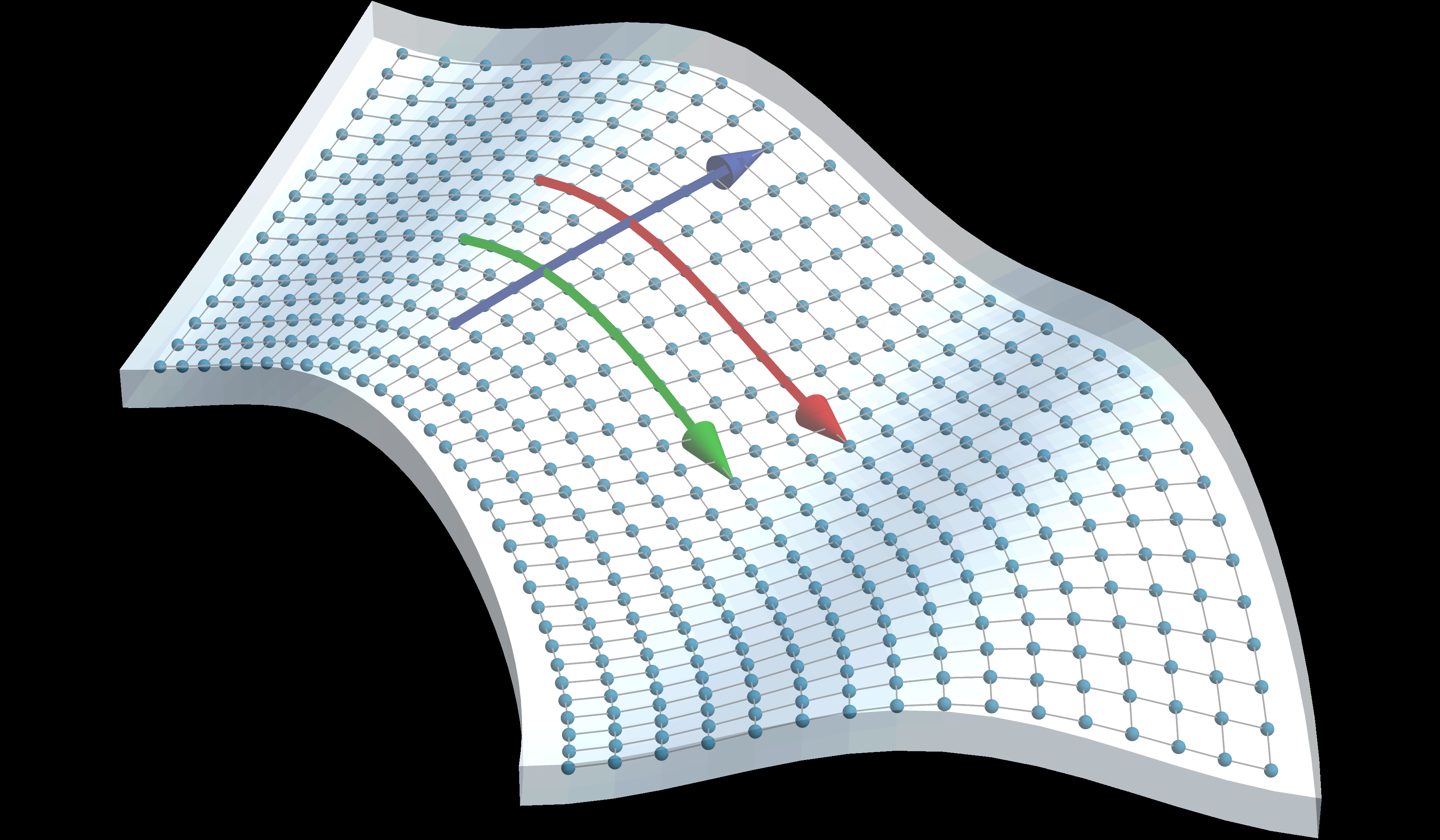
FIG. 1. Curvature induced nonlinear Hall effects. a Sketch of a curved ferromagnetic thin shell: the green and red arrows show the orientation of the magnetization M and of the driving electric field E, respectively. When the two vectors are parallel a second-harmonic transverse current J 2ω is observed induced by the quantum metric – the real part of the quantum geometric tensor (QGT) – of the electronic wavefunctions. b Momentum-space map of one of the three components of the band normalized quantum metric, namely Gx y , for a representative case. c Sketch of a bent ferromagnetic membrane with applied electric field E (red arrow) orthogonal to the magnetization M (green arrow). In this situation the second-harmonic transverse current J 2ω is parallel to the magnetization. This response is activated by the Berry curvature – the imaginary part of the QGT – whose density plot in momentum space is drawn in d. plane magnetization is perpendicular to the driving elec- tric field [see Fig. 1(c)]. This NAHE is induced by a curvature-induced BCD [see Fig. 1(d)] that is absent in the conventional flat material structure, and thus pro- vides a footprint of the imaginary part of the QGT. The curvature-induced NAHE we propose here rep- resents a new physical effect in curvilinear magnetism. Curvilinear magnetism has recently emerged as a power- ful approach to modify the magnetic state and thus the responses of magnetic materials. It has been originally conceived taking advantage of the coupling between the nanoscale shape of a magnetic structure and its magnetic order parameter [32–34]. Generally speaking, the con- finement of the magnetic energy functional to a bent two- dimensional surface is reflected in the appearance of an effective Dzyaloshinskii-Moriya interaction coupling and an effective anisotropy [35, 36]. The curvature-induced DMI has been shown, for instance, to stabilize modu- lated phases even in the complete absence of any materi- als’ intrinsic DMI [37]. Chiral responses stemming from the exchange-driven DMI have been experimentally ver- ified [38] using parabolic stripes of Ni8 1F e1 9 (Py). The exchange-induced anisotropy sets instead the magnetic ground state of systems with easy-surface type of magne- tocrystalline anistropy without any reorganization of the magnetic ground state. For example in one-dimensional rippled magnetic nanomebranes the stable ground state has a magnetization that is simply oriented perpendicular to the ripples and thus along the translationally invari- ant direction [39]. Our study demonstrates that despite this absence of curvature effects on the magnetic ground state, the real space geometry can generate non-trivial quantum geometric properties and yield intrinsic nonlin- ear transport phenomena. II. CURVATURE-INDUCED ORBITAL AND SPIN RASHBA COUPLING In this section we discuss how in quasi-two-dimensional (magnetic) metals geometric curvature leads to an or- bital Rashba coupling and, as a direct byproduct, to a spin-Rashba coupling. Let us start by considering a sin- gle valley system with orbital degrees of freedom. For

3 simplicity we will assume p orbitals but the same argu- ments apply also to the t2 g orbitals since they effectively span an effective angular momentum one subspace as the p orbitals. The corresponding energy spectrum is as- sumed to accurately represent the electronic bands close to the Fermi level of the (magnetic) metal in question. At the high-symmetry time-reversal invariant momentum around which the effective Hamiltonian is expanded and in the absence of geometric curvature, quantum confine- ment generally splits the three-dimensional irreducible representation (IRREP) corresponding to the atomic p orbitals into a one-dimensional IRREP a1 g and an eg doublet. To proceed further, let us obtain the effective Hamiltonian using the theory of invariants, which corre- sponds to a conventional k · p theory that keeps track of the point group symmetries of the crystal. To do so, we use that a generic three-band Hamiltonian can be ex- panded in terms of the nine Gell-Mann matrices [40] Λi as H(k) = 8 i=0 gi ( k)Λi (1) where Λ0 corresponds to the identity. The fact that the Hamiltonian must remain invariant requires that the momentum polynomials gi ( k) must belong to the same representation of the crystal point group of the corre- sponding Gell-Mann matrix. To make things concrete let us consider a crystalline systems with D4 h point group. The generators of the D4 h are a fourfold rotation C4 v , a twofold rotation C′2 with rotation axis orthogonal to the fourfold rotation axis, and the horizontal mirror σh . In Table 1 we list the representation of the Gell-Mann ma- trices in the px , py , pz orbital basis and momentum poly- nomials up to quadratic order in the D4 h point group. From this we find that the effective Hamiltonian away from the high-symmetry time-reversal invariant momen- tum reads Hk = ∆ Λ8 + γ0 Λ 0 k2x + k2y +γ3 k2x − k2y Λ3 + γ1 k x k y Λ1 , (2) where ∆ indicates the crystal field splitting, γ0 accounts for a conventional orbital independent while γ1 and γ3 parametrize d-wave orbital hybridization terms that yield orbital dependent effective masses. Let us now introduce geometric curvature in the thin film. It is well known [41] that across the thin film curvature introduces a strain field that varies linearly across the film with regions under compressive and tensile strain separated by a mechani- cally neutral plane [42, 43]. The consequence of the pres- ence of this strain field is twofold. First, the twofold ro- tation around the in-plane axis C′2 is broken. Second, and perhaps even more importantly, the thin film will not pos- sess any horizonal mirror symmetry. Therefore, even if the fourfold rotation symmetry is preserved, centrosym- metry is inevitably lost. The highest symmetry point group symmetry will thus be the polar C4 v group. This geometry-induced symmetry reduction strongly changes the electronic structure of our multiorbital system. In TABLE I. Character tablesa for the point groups D4 h and C4 v D4 h E C4 C′2 σh I polynomials of k Gell-Mann matrices A1 g 1 1 1 1 1 1, k2x + k2y Λ0 , Λ8 A2 g 1 1 −1 1 1 – Λ2 B1 g 1 −1 1 1 1 k2x − k2y Λ3 B2 g 1 −1 −1 1 1 kx k y Λ1 Eg 2 0 0 −2 2 – {Λ4 , Λ6 } {Λ5 , Λ7 } C4 v E C4 σv polynomials of k Gell-Mann matrices A1 1 1 1 1, k2x + k2y Λ0 , Λ8 A2 1 1 −1 – Λ2 B1 1 −1 1 k2x − k2y Λ3 B2 1 −1 −1 kx k y Λ1 E 2 0 0 {kx , ky } {Λ4 , Λ6 } {Λ5 , Λ7 } a For simplicity we only report the generators of the group. Additionally, we indicate the representation of the Gell-Mann matrices and the polynomials of momentum k in two dimensions. The model Hamiltonians reported in the main text can be obtained by additionally using the time-reversal symmetry constraint H⋆ (−kx , −ky ) = H(kx , ky ). fact, and as shown in Table 1, terms which are linear in momentum are allowed. The effective Hamiltonian up to linear order now reads Hk = ∆ Λ8 + γ0 Λ 0 k2x + k2y + αO R (kx Λ 5 + ky Λ7 ) , (3) where for simplicity we neglected the orbital hybridiza- tion terms quadratic in momentum, and the linear term gets the form of the so-called orbital Rashba cou- pling [29–31] kx L y −ky Lx [see the Methods section]. Note that kx ,y indicate now the momenta along the principal directions of the two-dimensional curved manifold. Im- portantly, the curvature-induced orbital Rashba coupling is transmuted in an effective Rashba spin-orbit coupling (SOC) term in materials with a non-negligible atomic SOC [see the Methods section]. As a result, the effective Hamiltonian for a Kramers’ doublet corresponds to the theory of a Rashba gas with an effective spin Hamiltonian Hs pin( k) = αR (kx σ y − ky σx ) + ℏ2 k2 2m⋆ σ0 (4) with the Rashba spin-orbit coupling strength αR that is directly proportional to curvature-induced orbital Rashba coupling both when the atomic SOC energy is much larger than the crystal field splitting ∆, and in the opposite weak spin-orbit coupling regime [see the Meth- ods section]. Having obtained the form of the effective Hamiltonian in a multiorbital system when geometric curvature de- creases the point group from D4 h to C4 v , we next explic- itly consider an effective model relevant for thin ferro- magnetic shells. In doing so, we notice that the exchange

4 coupling between the conducting electrons and the lo- calized magnetic moments can be a priori influenced by curvature effects on the long-range magnetic order. It is well-known [35, 36], in fact, that the magnetic energy functional in curved thin magnetic shell is endowed with a curvature-induced Dzyaloshinskii-Moriya interaction (DMI) and an effective magnetic anisotropy controlled by curvature. Generally speaking, these curvature-induced effects yield a reorganization of the magnetic texture. However, in a easy-surface magnetic nanomembrane such curvature-induced reorganization of the magnetic texture is absent [39]. Consequently, the magnetic order parame- ter is along the curved surface of the magnetic shell. The effective Hamiltonian for conduction electrons with the exchange coupling to localized moments then reads: Hs pin 1 (k) = αR (kx σ y − ky σx ) + ℏ2 k2 2m⋆ σ0 + M · σ (5) where M is the saturated magnetization and σ is the Pauli matrix vector. The Hamiltonian written above is universal and ap- plies to any three-dimensional geometric shape the easy- surface thin magnetic shell acquires. It also implicitly use the fact that there are no strain fields along the princi- pal in-plane curved directions. However, such inhomoge- neous strain fields, experimentally shown in corrugated bilayer graphene [17], are generally expected [see Fig. 1]. The presence of this strain fields can lead to a complete loss of rotational symmetries around the out-of-plane axis. This implies that the spin Hamiltonian possesses an additional symmetry-allowed term λky σz where we as- sumed a residual mirror symmetry My sending y → −y. The spin Hamiltonian in this case will read Hs pin 2 (k) = αR (kx σ y − ky σx ) + λky σz + ℏ2 k2 2m⋆ σ0 + M · σ (6) along the ˆx axis of the thin magnetic shell: recall that in the presence of bending ˆx corresponds to one of the principal direction of the curved membranes shape. For systems with an evenfold rotation symmetry in the non- magnetic phase, and thus described by Eq. (5), the mag- netic point group contains the combined M′y = My Θ symmetry with My the vertical mirror symmetry paral- lel to the magnetization, and a residual Mx symmetry. On the contrary systems described by Eq. (6) have a magnetic point group containing only My . Under both M′y and Mx we have that the crystalline momentum kx → −kx whereas ky → ky . By additionally using the transformation of the symmetric quantum metric tensor under the vertical mirror symmetry we then get that the following symmetry constraints gx x( kx , ky ) = gx x( −kx , ky ) gy y (kx , ky ) = gy y (−kx , ky ) (7) gx y (kx , ky ) = −gx y (−kx , ky ). Therefore, we can conclude that the properties of the quantum metric are independent of the specific model Hamiltonian choice. We next show how these symmetry-enforced properties of the quantum metric are reflected in the nonlinear elec- tron transport characteristics, specifically on the electric nonlinear anomalous Hall effect induced by the quantum metric. The latter is in fact governed by the dipoles of the band-energy normalzed quantum metric (BNQM) G± ab( kx , ky ) = ±ga b( kx , ky )/|d|, where the ± refers to the internal and external Rashba electronic branches respec- tively. Specifically we have that the intrinsic transversal nonlinear conductivity components [19–21] read σQ M a;bb = − e3 ℏ n d2 k (2π)2 Λna ;bb( k)fn ( k) (8) where n = ±, fn indicates the Fermi-Dirac distribution function, and the BNQM dipole densities

III. NONLINEAR ANOMALOUS HALL EFFECT DUE TO THE QUANTUM METRIC The end product of the crystalline symmetry break- ing due to bending is generally the spin-momentum lock- ing encoded in the Rashba spin-orbit coupling term of Eqs. (5),(6). It has been recently shown [26] that a prime physical consequence of spin-momentum locking is the fact that the corresponding Bloch waves are endowed with a non-trivial QGT. Importantly, the quantum met- ric is not forced to be vanishing at all momenta by the local in momentum C′2 symmetry. This implies that both the Hamiltonians in Eqs. (5),(6) have a non trivial QGT. Additionally, and as shown below, the symmetry proper- ties of the quantum metric are the same in both cases. The quantum metric is defined by ga b( kx , ky ) = ∂k a ˆd · ∂k b ˆd/4 where ˆd = d/|d| is the normalized Hamiltonian vector defined by Hs pin (k) = d·σ. Without loss of gener- ality, we fix the direction of the saturated magnetization Λ± a;bb( k) = 3 2 ∂a G ± bb( k) − ∂b G ± ab( k). (9) In Fig. 2 we show the momentum space maps of the two BNQM dipole densities governing the nonlinear anoma- lous Hall conductivities σy ;xx and σx ;yy assuming the model Hamiltonian in Eq. (5) – we refer to the Supple- mentary Information for an analogous discussion consid- ering Eq. (6). The BNQM dipole density Λy ;xx( k) is en- forced by symmetry to be an even function of the momen- tum kx and will thus generally provide a non-vanishing contribution to the nonlinear anomalous Hall conductiv- ity σy ;xx. The BNQM dipole Λx ;yy (k) instead is forced by symmetry to be an odd function of the momentum kx . Together with the fact that the electronic band energies ϵ± ( kx , ky ) = ϵ± ( −kx , ky ) by virtue of M′y and/or Mx we thus conclude that the non-trivial quantum metric does not a generate a nonlinear anomalous Hall conduc- tivity when the driving electric field is orthogonal to the

5 10 4

a c e ∂y Gx x ky kx ∂x Gx y ky kx Λy ;xx ky kx

c d f ∂x Gy y ky kx ∂y Gx y ky kx Λx ;y y ky kx 0 −10 −104 (a.u.)

FIG. 2. Band Normalized Quantum Metric Dipoles. a-d Contour plots of the band-normalized quantum metric (BNQM) dipoles ∂a G b c (with a, b, c, = x, y and ∂a ≡ ∂/∂k a ) in momentum space in arbitrary units (a.u.) for a representative set of parameters and for magnetization directed along ˆx. e-f Contour plots of the functions Λy ;xx( k) and Λx :yy (k), respectively, which are built as linear combination of BNQM dipoles (see equation (9)). Notice that Λy ;xx( k) is an even function of the momentum kx and will thus generally provide a non-vanishing contribution to the nonlinear anomalous Hall conductivity, while Λx ;yy (k) is an odd function of kx and the integration in k-space over the occupied state will vanish. in-plane magnetization. Similar symmetry constraints are also found when considering the extrinsic nonlinear Drude contribution that generally reads σN LD a ;bb = − e3 τ 2 ℏ3 n∈occ. d2 k (2π)2 ∂a ∂ b ∂ b ε n ( k)fn ( k), (10) where τ indicates the electronic scattering time. The band energy derivative ∂k x ∂k y ∂k y ϵ± ( k) is enforced to be an odd function of kx thus guaranteeing the absence of the nonlinear Drude contribution σN LD x ;yy . On the con- trary, the nonlinear Drude contribution σN LD y ;xx is not forced to vanish by symmetry and will thus coexist with the intrinsic quantum metric contribution discussed be- fore. Next, we discuss the behavior of the nonlinear Drude and the quantum metric-induced contributions to the nonlinear conductivity σy ;xx. First, we note that the energy spectrum of the model Hamiltonian in Eq. (5) features a crossing protected by Mx on the mirror sym- metric line kx = 0 [see Fig. 3(a)]. The finite ky value at which the crossing occurs is determined by kcy = M/αR and shifts away from the time-reversal invariant momen- tum as the magnetization increases. The corresponding crossing energy Ec = ℏ2 M 2 /(2m⋆ α2R ) identifies two dif- ferent regimes for the properties of the Fermi lines [see the Supplementary Information]. In fact, at Fermi energies EF > Ec the two Fermi lines corresponding to the two spin bands wind around the crossing point kc = 0, kcy . This winding does not occur for EF ≤ Ec . Additionally, in this regime we find the occurrence of a Lifshitz transi- tion determined by EF ≡ EL [see Fig. 3(a)] below which a single spin band is occupied [see also the Supplemen- tary Information]. In Fig. 3(b) we show the Fermi energy dependence of the intrinsic quantum metric induced nonlinear anoma- lous Hall conductivity term σQ M y ;xx. For EF < EL we find that σQ M y ;xx grows linearly with a slope that increases with the Rashba coupling α3R . At the Lifshitz transition, the nonlinear conductivity displays a kink that is followed by a much weaker and nonlinear Fermi energy dependence. By further increasing EF (see the Supplementary Infor- mation) one finds that the zero-temperature nonlinear conductivity is characterized by an asymptotic behavior at Ec that resembles the behavior of the nonlinear mag- netoconductivity σx ;xx in nonmagnetic two-dimensional electron gases [26]. The extrinsic nonlinear Drude contri- bution σN LD y ;xx is characterized by features [see Fig. 3(c)] which are very similar to σQ M y ;xx only in the EF < Ec regime. In fact, in the opposite EF > Ec regime the nonlinear Drude contribution vanishes thus making the

6 a d QM σ a;bb (μA nm V -2 )

E n E c E L 0.01 0.02 0.03 0.04 NLD σ y;xx (μ A nm V -2 )

QM σ y;xx (μ A nm V -2 ) α R (eV Å)

0.2 0.0 0.04 0.03 0.05 0.10 0.15 π 3 π 2 2 π 0.20 E F ( eV )

α R (eV Å)

0.01 0.02 0.03 0.04 0.02 0.01 0.00 0.00 π 2 0 c 0.4 σ y;xx σ x;yy -0.5 θ b 0.6 0.0 k y M α R 0.8 0.5 0.00 0.05 0.10 0.15 0.20

E F ( eV )

FIG. 3. Quantum metric induced nonlinear anomalous Hall effect. a Energy bands as a function of ky for kx = 0 when the magnetization M is in the ˆx direction. The dashed line marks the energy of the Lifshitz transition EL . The band-crossing occurs at (kx = 0; kcy = M/αR ) and Ec = ℏ2 M 2 /2m⋆ α2R . b Behavior of the quantum metric induced nonlinear conductivity tensor component σQ M y ;xx as a function of the Fermi energy EF for M = 40 ˆx meV and four different values of Rashba spin-orbit coupling αR (see legend). The kink in the behavior occurs for EF = EL . c Plot of the nonlinear Drude conductivity tensor component σN LD y ;xx for the same set of parameters of b and relaxation time τ = 10fs. d Plot of σQ M a ;bb (with {a, b} = {x, y}) as a function of the in plane orientation θ of the magnetization for M = 40meV, αR = 0.04eV˚A and EF = 80meV. The two components (y; xx) and (x; yy) are related by a π/2 shift and show a 2π-periodic non-sinusoidal behavior. anomalous Hall conductivity σy ;xx entirely intrinsic. Ad- ditionally, in the EF < Ec regime the two contributions can be parsed thanks to the different dependence on the electronic scattering time τ . The latter can be controlled using the temperature dependence of the linear conduc- tivity. Transport experiments at variable temperature will thus allow to single out the quantum metric-induced contribution to the nonlinear conductivity. In Fig. 3(d) we show the angular dependence of the in- trinsic conductivity σQ M y ;xx as obtained by tilting the mag- netic field direction from ˆx by a θ angle. We find that the nonlinear conductivity is 2π-periodic in agreement with the fact that σQ M y ;xx must be odd in the magnetization M . Additionally, due to the breaking of the Mx , M′y sym- metries the nonlinear conductivity σx ;yy acquires finite values at θ ̸= 0. However, the angular dependence of the two nonlinear conductivities are related to each other by a simple π/2 offset. This signals that, independent of the magnetization direction, when the driving electric field is collinear to the magnetization, only a transversal nonlin- ear current will be generated. We emphasize that this property is specific to our model Hamiltonian in Eq. (5), which, does not feature crystalline anisotropy terms and thus possess full rotational symmetry in the absence of magnetization [see also Supplementary Information]. IV. BERRY CURVATURE-INDUCED NONLINEAR ANOMALOUS HALL EFFECT In this section, we will show that thin magnetic shells where geometric deformations lead to a complete loss of rotational symmetries, there is an additional contribu- tion to the nonlinear Hall conductivity induced by the Berry curvature. We start by recalling that under a C2 rotation the out-of-plane component of the Berry cur- vature Ωz (kx , ky ) → Ωz (−kx , −ky ). Additionally, time- reversal symmetry sends kx ,y → −kx ,y and concomi- tantly reverse the Berry curvature Ωz → −Ωz . There- fore we obtain that the combined C′2 symmetry implies Ωz (kx , ky ) = −Ωz (kx , ky ) = 0. We note that C′2 is inher- ently present in systems described by the Hamiltonian in Eq. (5) thereby guaranteeing that the Berry curvature and its related transport effects cannot appear even if time-reversal symmetry is broken. For systems with a residual M′y symmetry, and thus

7 a 1.0 ϵ F (eV)

D x D y 0.001 0.02 0.03 0.04 D a (Å) D y (Å) D y (Å)

α R (eV Å )

0.003 0.0

M αR ky Ec En b c ∂y Ωz ky kx ∂x Ωz ky kx 102 10 0 −10 −102 (a.u.)

e d 0.002 0 0.08 0.12 0.16 -0.5

0.001

-1.0 0.00 0.05 0.10 0.15 0.20 0.25 0.30 0.000

0.00 0.05 0.10 0.15 0.20 0.25 0.30 α R (eV Å) λ (eV Å)

0 π 2 π 3 π 2 2 π

θ

FIG. 4. Berry curvature induced nonlinear anomalous Hall effect. a Energy bands as a function of ky for kx = 0 when the magnetization is in the ˆx direction and for λ ̸= 0. The coupling λ removes the degeneracy and, as reference, the (λ = 0)-energy bands are plotted in gray. b-c Contour plots of the k-space gradient of the Berry curvature ∂y Ωz and ∂y Ωz , respectively, for a representative set of parameters and M ∥ ˆx. d-e Behavior of the Berry curvature dipole (BCD) Dy as a function of the Rashba coupling αR and of parameter λ, respectively, for M = 40 ˆxmeV. In d the BCD is displayed for λ = 0.02eV˚A and for three different values of the Fermi energy. The BCD features a sign change and the double peak structure which occur for values of αR close to the condition EF = Ec . In e the Fermi energy is set to EF = 80meV and the BCD shows a non-monotonic behavior as a function of λ. In f the BCDs Dx and Dy are presented as a function of the angle θ formed by the magnetization M and the ˆx axis. The BCDs show a π-periodic behavior, in contrast with the quantum metric induced nonlinear conductivity. Notice that with the choice λky σz the Berry curvature is zero for θ = π/2. The parameters used here are M = 40meV, αR = 0.04eV˚A EF = 80meV, λ = 0.02eV˚A. described by the Hamiltonian in Eq. (6) with the satu- rated magnetization that is fixed again along the ˆx direc- tion, the situation is completely different. The effect of the λky σz term is twofold. First, it removes the mirror- symmetry protected crossing with the two spin bands that become non-degenerate at all k points [see Fig. 4(a)]. Second, it endows the system with a local Berry curva- ture with non-zero average. This also implies that, the system features an in-plane anomalous Hall effect, which represents the magnetic analog of the anomalous planar Hall effect predicted in two-dimensional systems [44, 45]. Perhaps even more importantly, the momentum depen- dence of the Berry curvature is characterized by a non- vanishing Berry curvature dipole [5–7] Dy = n d2 k (2π)2 ∂k y Ωnz (k)fn ( k). (11) The residual M′y symmetry implies in fact that the Berry curvature Ωnz ( kx , ky ) = Ωnz ( −kx , ky ). The dipole den- sity ∂k y Ωnz ( k) is consequently an even function of kx [see Fig. 4(b)], as the band energies are, thereby implying a non-vanishing dipole Dy . On the contrary, the dipole Dx is forced to vanish for the simple reason that its density [see Fig. 4(c)] is an odd function of kx . The behavior of the BCD Dy as a function of the Rashba spin orbit coupling constant αR is displayed in Fig. 4(d) for different values of the Fermi energy. It fea- tures a double-peak structure occurring when the Fermi energy sits in vicinity of the avoided level crossing at Ec . This is because in this region of near degeneracy the Bloch waves are rapidly changing, and thus produce hotspots of BC and BCD. Fig. 4(e) shows the behavior of Dy by increasing the strength of the mirror symme- try breaking term parametrized by λ. The dipole has a non-monotonic behavior and is maximized at a finite λ value that is weakly dependent on the Rashba spin- orbit coupling strength. The fact that the dipole dis- plays this non-monotonic dependence can be understood by noticing that in the λ → 0 limit, the dipole must van-

8 ish since the C2 Θ symmetry is restored. On the other hand, the dipole vanishes also in the λ → ∞ limit. This can be shown using the following argument: taking only the leading order terms, the Hamiltonian in Eq. (6) can be written as Hs pin 2 (k) ≃ αR k x σ y + M σx + λky σz + ℏ2 k2 2m⋆ σ0 (12) The first three terms in the equation above, which deter- mine the Berry curvature, describe an anisotropic mas- sive Dirac cone with Fermi velocities αR and λ and mass given by the magnetization M . The corresponding Berry curvature becomes strongly peaked at ky = 0 as the related velocity λ increases, which justifies the use of Eq. (12) in the λ → ∞ limit. Furthermore, both the approximate Berry curvature and the band energies be- come even functions of the momentum ky thereby imply- ing that the corresponding dipole Dy must vanish. The existence of a finite Berry curvature dipole Dy at finite values is reflected in the appearance of a non- vanishing nonlinear conductivity σx ;yy = e3 τ /ℏ2 Dy . Note that the linear in τ dependence is required in or- der to have a σx ;yy compatible with the M′y symmetry. The linear dependence in the relaxation time also implies that the magnetization dependence of σx ;yy must be an even function, contrary to σy ;xx that is odd in M. As a result, a swap of the magnetization does not change the Berry curvature dipole-induced nonlinear conductiv- ity. This is immediately demonstrated in Fig. 4(f) where we show the behavior of the dipole Dy by changing the magnetization angle with respect to the ˆx axis. We have that the Berry curvature dipole has a π periodicity. Note that when the magnetization direction θ ̸= 0 the Berry curvature dipole acquires a ˆx component. Both dipoles however disappear at θ ≡ π/2. This is due to the fact that in this configuration the system preserves the verti- cal mirror symmetry My and a crossing on the ky = 0 mirror symmetric line will therefore occur. The Berry curvature itself in this situation will therefore vanish. V. CONCLUSIONS To wrap up, we have shown that easy-surface thin fer- romagnetic shells even of centrosymmetric materials will display a nonlinear anomalous Hall effect when acquiring curved geometric shapes. Despite the absence of cur- vature effects on the magnetic order parameter, curva- ture drives non-trivial quantum geometric properties of the Bloch waves via the occurrence of spin-momentum locked textures. We have shown that when undergoing bending, easy-surface ferromagnetic shells will then dis- play a nonlinear anomalous Hall effect that is maximized when the driving electric field is collinear to the saturated magnetization. Additionally, whenever geometric defor- mations lead to a complete rotational symmetry breaking a complementary nonlinear anomalous Hall effect due to the Berry curvature dipole can be observed when the driving electric field is orthogonal to the magnetization. The combination of these two effects therefore allow to obtain a complete mapping of the quantum geometric tensor using nonlinear transport experiments. Our the- oretical study thus shows real-space geometric control of the quantum geometric properties of the electronic wave- functions in magnetic materials and highlights a novel spin-orbitronic effect in magnetic nanomembranes. VI. METHODS A. Representation of the Gell-Mann matrices The eight Gell-Mann matrices can be defined as Λ1 = 0 1 0 1 0 0 0 0 0 , Λ2 = 0 −i 0 i 0 0 0 0 0 , Λ3 = 1 0 0 0 −1 0 0 0 0 , Λ4 = 0 0 1 0 0 0 1 0 0 , Λ5 = 0 0 −i 0 0 0 i 0 0 , Λ6 = 0 0 0 0 0 1 0 1 0 , Λ7 = 0 0 0 0 0 −i 0 i 0 , Λ8 = 1√ 3 0 0 0 1√ 3 0 0 0 −2√ 3 . B. Derivation of the Rashba Hamiltonian To derive an effective spin Hamiltonian, we first note that the conventional angular momentum operators are related to the Gell-Mann matrices introduced above by Λ2 = Lz , Λ7 = Lx , and Λ5 = −Ly . This implies that the term linear in momentum in the Hamiltonian of Eq. (3) can be written as HO R = αO R( kx L y − ky Lx ) . (13) Let us now include the spin-orbit coupling term in the Hamiltonian HS O = λS OC L · S = λS OC α=x,y,z Lα σ α / 2. In the weak crystal field split- ting regime ∆ ≪ λS OC , we have that that the spin-orbit coupling splits the (effective) p-orbital manifold into a J = 3/2 quartet at energy +λS OC /2 and a J = 1/2 doublet at energy −λS OC . The total energy splitting is therefore ∆ = E3 /2 − E1 /2 = 3 2 λS OC . We next derive the effective low-energy model for the J = 1/2 doublet. To this aim, we recal that that |J, Jz ⟩ states can be expressesed in terms of the |L, Lz ⟩ ⊗ |σ, σz ⟩ states using

9 the Clebsch-Gordan coefficients as 1 2 , + 1 2 = 2 3 |1, 1⟩ 1 2 , − 1 2 − 1 3 |1, 0⟩ 1 2 , 1 2 , 1 2 , − 1 2 = 2 3 |1, −1⟩ 1 2 , 1 2 − 1 3 |1, 0⟩ 1 2 , − 1 2 . with the angular momentum eigenstates that are related to the atomic real orbitals by |1, ±1⟩ = ∓(px ± ipy )/ √2 and |1, 0⟩ = pz . The two states composing the J = 1/2 doublet |1/2, ±1/2⟩ are related to the real orbitals by 1 2 , + 1 2 = − 1√3 (pz | ↑⟩ + px | ↓⟩ + i py | ↓⟩) 1 2 , − 1 2 = − 1√3 (pz | ↓⟩ − px | ↑⟩ + i py | ↑⟩) Let us now introduce the effective spin-1/2 operator τ spanning the J = 1/2 space. By evaluating the angular momentum operators over the states introduces above we have that in the J = 1/2 basis Li → 1 3 τi . Note that the projection of terms of the form Li L j (which include the orbital hybridization terms quadratic in momentum) can be expressed as Li L j → 19 τi τ j which however yields only an identity term in the effective Hamiltonian as a result of the relation for the Pauli matrices τα τ β = δα β + i ϵα βγ τγ with δα β the Kronecker delta. As a result, we have that in the strong spin-orbit coupling regime the effective Hamiltonian reads Rashba spin-orbit coupling can be also seen in the op- posite limit in which the atomic spin-orbit couplins is considered as a perturbation. In this case, we consider the full Hamiltonian as HT = Hk + HS O with Hk corre- sponding to Eq. (3) of the main text. In this case, the effect of spin-orbit coupling can be taken into account by performing a Schrieffer-Wolff transformation and de- ducing the effective spin Hamiltonian for the spin-one- half doublet with pz orbital character. Then the effective Hamiltonian Hs pin( k) = h ⟨ℓ|HS O| h⟩⟨h|Hk | ℓ⟩ + h.c. Eℓ − Eh (15) where the |ℓ⟩ = px |↑, ↓⟩ while |h⟩ is the quartet of degen- erate states related to the px , py orbitals. The final form of the effective spin-Hamiltonian is Hs pin( k) = 2λS OC αO R ∆ (kx σ y − ky σx ) + ℏ2 k2 2m⋆ σ0 with σ0 the identity matrix. ACKNOWLEDGMENTS M.C. acknowledges partial support by Italian Ministry of University and Research (MUR) PRIN 2022 under the Grant No. 2022LP5K7 (BEAT) and from PNRR MUR project PE0000023-NQSTI. M.T.M. and C.O. ac-

only an identity term in the effective Hamiltonian as a result of the relation for the Pauli matrices τα τ β = δα β + i ϵα βγ τγ with δα β the Kronecker delta. As a result, we have that in the strong spin-orbit coupling regime the effective Hamiltonian reads ˜H = 1 3 αO R( kx τ y − ky τx ) (14) with the characteristic Rashba spin-orbit coupling strength that is a third of the orbital Rashba coupling. That the concomitant presence of orbital Rashba cou- pling and spin-orbit coupling gives rise to an effective M.C. acknowledges partial support by Italian Ministry of University and Research (MUR) PRIN 2022 under the Grant No. 2022LP5K7 (BEAT) and from PNRR MUR project PE0000023-NQSTI. M.T.M. and C.O. ac- knowledge partial support from PNRR MUR Project No. PE0000023-NQSTI (TOPQIN). Author contributions: All authors contributed ex- tensively to the work presented in the paper. Competing interests: The authors declare that there are no competing financial or non-financial inter- ests. [1] Provost, J. P. & Vallee, G. Riemannian structure on manifolds of quantum states. Communications in Math- ematical Physics 76, 289–301 (1980). [2] Thouless, D. J., Kohmoto, M., Nightingale, M. P. & den Nijs, M. Quantized Hall conductance in a two- dimensional periodic potential. Phys. Rev. Lett. 49, 405– 408 (1982). URL https://link.aps.org/doi/10.1103/ PhysRevLett.49.405. fect induced by Berry curvature dipole in time-reversal invariant materials. Phys. Rev. Lett. 115, 216806 (2015). URL https://link.aps.org/doi/10.1103/ PhysRevLett.115.216806. [6] Ortix, C. Nonlinear Hall effect with time-reversal sym- metry: Theory and material realizations. Advanced Quantum Technologies 4, 2100056 (2021). URL https: //doi.org/10.1002/qute.202100056.

˜H = 1 3 αO R( kx τ y − ky τx ) (14) with the characteristic Rashba spin-orbit coupling strength that is a third of the orbital Rashba coupling. That the concomitant presence of orbital Rashba cou- pling and spin-orbit coupling gives rise to an effective knowledge partial support from PNRR MUR Project No. PE0000023-NQSTI (TOPQIN). Author contributions: All authors contributed ex- tensively to the work presented in the paper. Competing interests: The authors declare that there are no competing financial or non-financial inter- ests. [1] Provost, J. P. & Vallee, G. Riemannian structure on manifolds of quantum states. Communications in Math- ematical Physics 76, 289–301 (1980). [2] Thouless, D. J., Kohmoto, M., Nightingale, M. P. & den Nijs, M. Quantized Hall conductance in a two- dimensional periodic potential. Phys. Rev. Lett. 49, 405– 408 (1982). URL https://link.aps.org/doi/10.1103/ PhysRevLett.49.405. [3] Haldane, F. D. M. Berry curvature on the Fermi surface: Anomalous Hall effect as a topological Fermi-liquid prop- erty. Phys. Rev. Lett. 93, 206602 (2004). URL https:// link.aps.org/doi/10.1103/PhysRevLett.93.206602. [4] Nagaosa, N., Sinova, J., Onoda, S., MacDonald, A. H. & Ong, N. P. Anomalous Hall effect. Rev. Mod. Phys. 82, 1539–1592 (2010). URL https://link.aps.org/doi/ 10.1103/RevModPhys.82.1539. [5] Sodemann, I. & Fu, L. Quantum nonlinear Hall ef- fect induced by Berry curvature dipole in time-reversal invariant materials. Phys. Rev. Lett. 115, 216806 (2015). URL https://link.aps.org/doi/10.1103/ PhysRevLett.115.216806. [6] Ortix, C. Nonlinear Hall effect with time-reversal sym- metry: Theory and material realizations. Advanced Quantum Technologies 4, 2100056 (2021). URL https: //doi.org/10.1002/qute.202100056. [7] Du, Z. Z., Lu, H.-Z. & Xie, X. C. Nonlinear Hall effects. Nature Reviews Physics 3, 744–752 (2021). URL https: //doi.org/10.1038/s42254-021-00359-6. [8] Su´arez-Rodr´ıguez, M. et al. Nonlinear transport in non-centrosymmetric systems. Nature Materials 24, 1005–1018 (2025). URL https://doi.org/10.1038/ s41563-025-02261-3. [9] He, P. et al. Quantum frequency doubling in the topological insulator Bi2 S e3 . Nature Communications

10
12, 698 (2021). URL https://doi.org/10.1038/ articles/s41586-023-06363-3.
s41467-021-20983-1. [26] Sala, G. et al. The quantum metric of electrons
s41467-021-20983-1.
[10] Makushko, P. et al. A tunable room-temperature non-
linear Hall effect in elemental bismuth thin films. Na-
ture Electronics 7, 207–215 (2024). URL http://dx.
doi.org/10.1038/s41928-024-01118-y.
[11] Isobe, H., Xu, S.-Y. & Fu, L. High-frequency recti-
fication via chiral bloch electrons. Science Advances
6 (2020). URL https://advances.sciencemag.org/
content/6/13/eaay2497.
[12] Hsieh, T. H. et al. Topological crystalline insulators in
the SnTe material class. Nature Communications 3, 982
(2012). URL https://doi.org/10.1038/ncomms1969.
[13] Lau, A. & Ortix, C. Topological semimetals in the SnTe
material class: Nodal lines and Weyl points. Phys. Rev.
Lett. 122, 186801 (2019). URL https://link.aps.org/
doi/10.1103/PhysRevLett.122.186801.
[14] Ma, Q. et al. Observation of the nonlinear Hall ef-
fect under time-reversal-symmetric conditions. Nature
565, 337–342 (2019). URL https://doi.org/10.1038/
s41586-018-0807-6.

s41586-018-0807-6. [15] Kang, K., Li, T., Sohn, E., Shan, J. & Mak, K. F. Non- linear anomalous Hall effect in few-layer WTe2 . Nature Materials 18, 324–328 (2019). URL https://doi.org/ 10.1038/s41563-019-0294-7.

10.1038/s41563-019-0294-7.
[16] Battilomo, R., Scopigno, N. & Ortix, C. Berry curvature
dipole in strained graphene: A Fermi surface warping ef-
fect. Phys. Rev. Lett. 123, 196403 (2019). URL https://

link.aps.org/doi/10.1103/PhysRevLett.123.196403.

link.aps.org/doi/10.1103/PhysRevLett.123.196403.
[17] Ho, S.-C. et al. Hall effects in artificially corrugated
bilayer graphene without breaking time-reversal sym-
metry. Nature Electronics 4, 116–125 (2021). URL

https://doi.org/10.1038/s41928-021-00537-5.

https://doi.org/10.1038/s41928-021-00537-5.
[18] Lesne, E. et al. Designing spin and orbital sources of
Berry curvature at oxide interfaces. Nature Materials
22, 576–582 (2023). URL https://doi.org/10.1038/
s41563-023-01498-0.
s41563-023-01498-0.
[19] Gao, Y., Yang, S. A. & Niu, Q. Field induced positional
shift of Bloch electrons and its dynamical implications.
Phys. Rev. Lett. 112, 166601 (2014). URL https://

link.aps.org/doi/10.1103/PhysRevLett.112.166601.

link.aps.org/doi/10.1103/PhysRevLett.112.166601.
[20] Das, K., Lahiri, S., Atencia, R. B., Culcer, D. &
Agarwal, A. Intrinsic nonlinear conductivities in-
duced by the quantum metric. Phys. Rev. B 108,
L201405 (2023). URL https://link.aps.org/doi/10.
1103/PhysRevB.108.L201405.
[21] Kaplan, D., Holder, T. & Yan, B. Unification of nonlin-
ear anomalous Hall effect and nonreciprocal magnetore-
sistance in metals by the quantum geometry. Phys. Rev.
Lett. 132, 026301 (2024). URL https://link.aps.org/
doi/10.1103/PhysRevLett.132.026301.
[22] Jiang, Y., Holder, T. & Yan, B. Revealing quantum
geometry in nonlinear quantum materials. Reports on
Progress in Physics 88, 076502 (2025). URL https://
doi.org/10.1088/1361-6633/ade454.
[23] T¨orm¨a, P. Essay: Where can quantum geometry lead
us? Phys. Rev. Lett. 131, 240001 (2023). URL https://

link.aps.org/doi/10.1103/PhysRevLett.131.240001.

link.aps.org/doi/10.1103/PhysRevLett.131.240001.
[24] Gao, A. et al. Quantum metric nonlinear Hall effect in
a topological antiferromagnetic heterostructure. Science
381, 181–186 (2023).
[25] Wang, N. et al. Quantum-metric-induced nonlinear
transport in a topological antiferromagnet. Nature
621, 487–492 (2023). URL https://www.nature.com/
articles/s41586-023-06363-3.
[26] Sala, G. et al. The quantum metric of electrons
with spin-momentum locking. Science 389, 822–825
(2025). URL https://www.science.org/doi/abs/10.
1126/science.adq3255.
[27] Mercaldo, M. T., Cuoco, M. & Ortix, C. Nonlinear planar
magnetotransport as a probe of the topology of surface
states. Phys. Rev. B 111, 155442 (2025). URL https:

//link.aps.org/doi/10.1103/PhysRevB.111.155442.

//link.aps.org/doi/10.1103/PhysRevB.111.155442.
[28] Sala, G. et al. Probing the quantum metric of 3d topo-
logical insulators (2026). URL https://arxiv.org/abs/
2509.17135. 2509.17135.
[29] Park, S. R., Kim, C. H., Yu, J., Han, J. H. & Kim,
C. Orbital-angular-momentum based origin of Rashba-
type surface band splitting. Phys. Rev. Lett. 107, 156803
(2011). URL https://doi.org/10.1103/PhysRevLett.
107.156803.
107.156803.
[30] B. Kim, B. et al. Microscopic mechanism for asym-
metric charge distribution in Rashba-type surface states
and the origin of the energy splitting scale. Phys. Rev.
B 88, 205408 (2013). URL https://doi.org/10.1103/
PhysRevB.88.205408.
PhysRevB.88.205408.
[31] Mercaldo, M. T., Solinas, P., Giazotto, F. & Cuoco,
M. Electrically tunable superconductivity through
surface orbital polarization. Phys. Rev. Applied
14, 034041 (2020). URL https://doi.org/10.1103/
PhysRevApplied.14.034041.
[32] Streubel, R. et al. Magnetism in curved geometries (Top-

ical Review). Journal of Physics D: Applied Physics

ical Review). Journal of Physics D: Applied Physics
49, 363001 (2016). URL https://doi.org/10.1088/

0022-3727/49/36/363001.

0022-3727/49/36/363001.
[33] Sheka, D. D. A perspective on curvilinear magnetism.
Applied Physics Letters 118, 230502 (2021). URL https:
//doi.org/10.1063/5.0048891.
[34] Makarov, D. et al. New dimension in magnetism and su-
perconductivity: 3D and curvilinear nanoarchitectures.
Advanced Materials 34, 2101758 (2022). URL https:
//doi.org/10.1002/adma.202101758.
[35] Gaididei, Y., Kravchuk, V. P. & Sheka, D. D. Curvature
effects in thin magnetic shells. Physical Review Letters
112, 257203 (2014). URL http://link.aps.org/doi/
10.1103/PhysRevLett.112.257203.
[36] Kravchuk, V. P. et al. Topologically stable mag-
netization states on a spherical shell: Curvature-
stabilized skyrmions. Physical Review B 94, 144402
(2016). URL http://link.aps.org/doi/10.1103/
PhysRevB.94.144402.
PhysRevB.94.144402.
[37] Yershov, K. V., Kravchuk, V. P., Sheka, D. D. & R¨ossler,
U. K. Curvature effects on phase transitions in chiral
magnets. SciPost Phys. 9, 043 (2020). URL https://

scipost.org/10.21468/SciPostPhys.9.4.043.

scipost.org/10.21468/SciPostPhys.9.4.043.
[38] Volkov, O. M. et al. Experimental observation of
exchange-driven chiral effects in curvilinear magnetism.
Physical Review Letters 123, 077201 (2019). URL https:

//doi.org/10.1103/PhysRevLett.123.077201.

//doi.org/10.1103/PhysRevLett.123.077201.
[39] Ortix, C. & van den Brink, J. Magnetoelectric-
ity induced by rippling of magnetic nanomembranes
and wires. Physical Review Research 5, L022063
(2023). URL https://link.aps.org/doi/10.1103/
PhysRevResearch.5.L022063.
[40] Mercaldo, M. T., Noce, C., Caviglia, A. D., Cuoco, M.
& Ortix, C. Orbital design of Berry curvature: pinch
points and giant dipoles induced by crystal fields. npj

Quantum Materials 8, 12 (2023). URL https://doi.

11

org/10.1038/s41535-023-00545-y. [44] Battilomo, R., Scopigno, N. & Ortix, C. Anomalous pla-
[41] Landau, L. D. & Lifshitz, E. M. Theory of Elasticity, nar hall effect in two-dimensional trigonal crystals. Phys.
vol. 7 of Course of Theoretical Physics (Pergamon Press, Rev. Res. 3, L012006 (2021). URL https://link.aps.
Oxford, 1986), 3rd edn. org/doi/10.1103/PhysRevResearch.3.L012006.
[42] Ortix, C., Kiravittaya, S., Schmidt, O. G. & van den [45] Cullen, J. H., Bhalla, P., Marcellina, E., Hamilton, A. R.
Brink, J. Curvature-induced geometric potential in & Culcer, D. Generating a topological anomalous hall
strain-driven nanostructures. Phys. Rev. B 84, 045438 effect in a nonmagnetic conductor: An in-plane magnetic
(2011). URL https://link.aps.org/doi/10.1103/ field as a direct probe of the berry curvature. Phys. Rev.
PhysRevB.84.045438. Lett. 126, 256601 (2021). URL https://link.aps.org/
[43] Stengel, M. Microscopic response to gradient deforma- doi/10.1103/PhysRevLett.126.256601.
tions in insulators. Nature Communications 4, 2693
(2013). URL https://doi.org/10.1038/ncomms3693.

Supplementary Information for: “Curvature-induced nonlinear anomalous Hall effect in thin magnetic shells”

Maria Teresa Mercaldo,1 Mario Cuoco,2 and Carmine Ortix1 , 2

1 Dipartimento di Fisica “E. R. Caianiello”, Università di Salerno, IT-84084 Fisciano (SA), Italy

2 CNR-SPIN, c/o Università di Salerno, IT-84084 Fisciano (SA), Italy

1. QUANTUM METRIC CONTRIBUTION TO NON LINEAR CONDUCTIVITY

In this note we discuss in detail the behavior of the nonlinear conductivity contributions driven by the quantum metric in a noncentrosymmetric two-dimensional ferromagnet described by Rashba spin–orbit interaction and a uni- form magnetization. The second order intrinsic nonlinear conductivity is governed by the band normalized quantum metric (BNQM) dipoles Gna b. Indeed we have σQ M a;bc = − e3 ℏ n (occupied) d2 k (2π)2 Λna ;bc( k)fn ( k), (1) where fn ( k) = f (εn ( k)) is the equilibrium Fermi-Dirac distribution function of the n-band and a, b, c are cartesian coordinates and the functions Λa ;bc in the integral are expressed in term of first derivatives of the BNQM Gna b: Λna ;bc( k) = 3 2 ∂a G b c n − 1 2 (∂b G nc a + ∂c G na b) , (2) where ∂a ≡ ∂/∂ka . In the following, we consider separately the model Hamiltonians Hs pin 1 ,2 , introduced in Eqs.(5)-(6) of the main text, which capture different symmetry properties of the system.

A. C 2 Θ symmetric systems

We start by analyzing the transverse components of the conductivity tensor for the model Hamiltonian in Eq.(5) of the main text, i.e. Hs pin 1 (k) = αR (kx σ y − ky σx ) + ℏ2 k2 2m⋆ σ0 + M · σ (3) For this model, and limiting ourselves to transverse transport, we have: Λ±x ;yy (k) = 3 2 ∂x G ±y y − ∂y G±x y = ∓ α3R ( αR k x + M sin θ)[7(αR k x + M sin θ)2 + 2(αR k y − M cos θ)2 ] 8[(αR k x + M sin θ)2 + (αR k y − M cos θ)2 ]7 /2 (4) Λ±y ;xx( k) = 3 2 ∂y G±x x − ∂x G ±x y = ∓ α3R ( αR k y − M cos θ)[2(αR k x + M sin θ)2 + 7(αR k y − M cos θ)2 8[(αR k x + M sin θ)2 + (αR k y − M cos θ)2 ]7 /2 (5) The energy bands of the spin Hamiltonian (3) are shown in Fig.3a of main paper, while in Fig.S1 we show the Fermi contours for a representative set of parameters. There is a band crossing at energy: Ec = ℏ2 M 2 2m∗ α2R (6) which occurs at (kx , ky ) = (−M sin θ/αR , M cos θ/αR ) or, at k = M/αR for ϕ = π/2 + θ, using polar coordinates (k, ϕ) (see Fig. S 1(a)). We can distinguish two regimes in the properties of the Fermi contours, separated by the band-crossing energy. For EF > Ec , the Fermi lines wind around the crossing point, whereas for EF < Ec they encircle regions away from this point. Remarkably, in the former case it is possible to obtain an exact analytical expression for the nonlinear conductivity tensor σQ M a,bb . In contrast, for EF < Ec , analytical expressions can only derived in the approximation M ≫ αR k F , which is nevertheless the parameter regime relevant for the present study.

2 M

0 1 2 θ ϕ x M θ 0 1 y ( 1 / n m )

ky 2

(a) -2 -1 0 1 2 -2 -1 kx (1/nm) k (b) -2 -1 0 -2 -1 kx (1/nm) k y

Fig. S 1. (a) Fermi contours for αR = 0.2eV˚A, M = 40meV and EF = Ec = 160meV. The band crossing occurs at kc = M/αR = 2(1/nm) and ϕ = π/2 + θ. (b) Fermi lines for αR = 0.04eV ˚A, M = 40meV, EF = 80meV and θ = 0. For this values of the parameters Ec = 4eV. The dashed lines are the circular lines obtained for αR = 0, which can be used for obtaining analytical approximations in when M ≫ αR k F . Regime 1: EF < Ec . We start our analysis with the case in which the ratio αR k F /M ≪ 1. Thus the Fermi contours can be approximated with circular lines of equations ℏ2 k2 2m∗ ± M = EF , which is a zero order approximation in αR k F /M (see also Fig. S 1(b)). We next expand the functions Λa ,bb to leading order in αR k F /M , obtaining: Λ−y ;xx( k) = − α3R 16M 4 (9 + 5 cos(2θ)) cos θ + O αR k M (7) Λ−x ;yy (k) = − α3R 16M 4 (9 − 5 cos(2θ)) sin θ + O αR k M (8) Let’s start analyzing the case θ = 0. To evaluate σQ M y ,xx we have to distinguish wether the Fermi energy is below or above the energy EL associated to the Lifshitz transition (i.e. we distinguish situations in which only the first band is occupied and that where both bands are occupied). Indeed, in the first case we have to integrate Λ( −) y ,xx( k) on a circle up to kF − = (M + EF )/c2 (where c2 ≡ ℏ2 /(2m∗ )), while in the latter case (considering that Λ( +) = −Λ( −) , the integration is in the Fermi annulus between kF + = (EF − M )/c2 and kF − . The Lifshitz transition occurs exaclty at the energy of the band-crossing EL = Ec for M ≤ α2R / (2c2 ) , while for M > α2R / (2c2 ) – which is the situation we are studying – we have EL = M − α2R / 4c2 . Thus, in the present approximation we can consider EL ≃ M . Notice that at this order of approximation, the functions Λa ,bb do not depend on k, thus the momentum integration will give simply the area enclosed in the Fermi lines: for EF < EL the result will be proportional to k2F + = (M + EF )/c2 , while for EF > EL we will have the area of the annulus (i.e ∝ (k2F + − k2F − ) = 2M/c2 ) . Specifically, we find σQ M y ;xx = e2 ℏ 7 32π α3R M 4 2m∗ ℏ2 (M + EF ) for EF < EL (9) σQ M y ;xx = e2 ℏ 7 16π α3R M 3 2m∗ ℏ2 for EF > EL . (10) The comparison between the numerical results and the analytical approximation is shown in Fig. S 2. In panel (a), for the smallest values of αR , we clearly observe linear behavior while varying EF up to the Lifshitz transition, followed by a constant regime. Conversely, for the highest value of αR , deviations from this zero order approximation become visible. While the analytical model could be improved by including second-order corrections in αR k F /M (noting that first-order corrections vanish), such an expansion is not relevant to understand the origin of the cusp.

3 αR ( e VÅ ) 0.008 0.012 0.016 0.020 0.08 0.10 V - 2 ) σy ;xx σx ;yy 0.05 0.10 V - 2 ) (a) (b)

QM σ a;bb (μA nm σ y;xx (μ A nm

0.06 0.04

-0.05

0.02

-0.10 0.00 0.00 0.05 π

2 0 0.10 E F ( eV )

π 3 π 2 2 π θ

Fig. S 2. (a)-(b) Comparison between analytical and numerical results. The analytical functions are drawn with black dashed lines. In (a) we show the behavior of σQ M y ;xx as a function of EF . Here the analytical function is given by Eqs.(9)-(10) and EL ≃ M = 0.04eV. In (b) we show he comparison with the analytical expressions (11)-(12) of the angular behavior of the conductivity tensor components σQ M a ;bb (θ) for M = 40meV, αR = 0.02eV ˚A and EF = 60mev. For θ ̸= 0, considering EF > EL , we obtain: σQ M y ;xx = + e3 ℏ 1 32π α3R M 3 2m∗ ℏ (9 + 5 cos(2θ)) cos θ (11) σQ M x ;yy = − e3 ℏ 1 32π α3R M 3 2m∗ ℏ (9 − 5 cos(2θ)) sin θ. (12) The comparison of the angular behavior is shown in Fig. S 2(b). For completeness, in Fig. S 3 we show the behavior of the intrinsic contribution to conductivity σQ M y ;xx for EF < Ec for larger values of the Rashba parameter αR , where the expansion in αR k F /M is no longer valid. When λ = 0, we see a divergence for EF → Ec .

1.2 QM σ y;xx ( mA nm V -2 )

1000 1.0

0.8

0.6 α R (eV Å)

0.16 0.18 0.20

0.4 0.00

Fig. S 3. σQ M y ;xx as a function of EF for M = 40meV. There is cusp in the behavior of the conductivity which occurs at the Lifshitz transition. Here we clearly see that this point depends also αR . For αR = 0.02eV˚A, the en- ergy of the crossing point is at Ec = 0.16eV.

10 1 0.1 0.1 0.2

0.0 100 0.16 0.05 0.10 0.15 E F ( eV )

Regime 2: EF > Ec For this analysis we follow the strategy discussed in the Supplementary Information of Ref.[1]. Indeed, in this case it is convenient to introduce shifted momenta px = kx + M αR sin θ and py = ky − M αR cos θ, so that the Hamiltonian d-vector simplifies to d = (−αR p y , αR p x , 0). The advantage is that the BNQM-components, and hence their dipoles, do not depend on M . In particular we have: G±x x = ± p2y 4|αR | p5 , G±x y = ∓ px p y 4|αR | p5 , G±y y = ± p2x 4|αR | p5 (13) with p2 = p2x + p2y , and for the Λa ;bb- functions: Λ±y ;xx = ∓ py (2p2x + 7p2y ) 8|αR | p7 , Λ±x ;yy = ∓ px ( 7p2x + 2p2y ) 8|αR | p7 . (14)

4 0.06 0.06 2 2 (a) (b) (c) (d)

-2 -1 0 1 2 0.00 0.02 E -2 -1 0 1 2 0.00 0.02 E -2 -1 0 1 2 -2 -1 0 py ϕ pF 1 pF 2 -2 -1 0 py

-1 0 1 2 -2 -1 0 1 2 -2 -1 0 1 py ϕ pF 1 pF 2 -2 -1 0 1 2 -2 -1 0 1 py ϕ

p x

Fig. S 4. (a)-(b) Energy bands for a representative set of parameters (specifically: M = 12meV and αR = 0.16eV˚A), as a function of px , with py = 0 in (a) and as a function of py for px = 0 in (b). In the plots energy are in eV and momenta in (1/nm). The red dotted line shows the energy of the bands-crossing Ec , which in shifted momentum space occurs at the origin (px = 0, py = 0). In the inset in (b) we display the Fermi lines at E = Ec . (c)-(d) Fermi lines for two different values of Fermi energy, which are marked by the gray dashed lines in panels (a)-(b). We notice that in (c), which corresponds regime 2 (EF > Ec ) , for each value of ϕ ∈ [0, 2π] we will have one solution pF i for each Fermi contour, while in (d), corresponding to regime 1, the Fermi lines are not winding around the origin. Thus, there are values of the angle ϕ for which there are two solutions and values for which there are none. Indeed, as we can clearly see in panel (a), the lowest energy gray line does not intercept the energy bands along the py = 0 line. The dependence on M will appear in the conductivity tensor from the M -dependence of the Fermi contours. Indeed, using shifted momenta, the energy reads E± = ℏ2 2m∗ p2 + M 2 α2R + 2M p sin(ϕ − θ) αR ± |αR | p (15) and the degeneracy point will be always at the origin (px = 0, py = 0). In the present regime, EF > Ec , we have that both Fermi lines wind around the origin (px = 0, py = 0) of the shifted-momentum space, as shown in Fig. S 4(c). So, for any ϕ we find a value for the Fermi wave-vector pF (1,2)( ϕ). Instead, for EF < Ec , i.e. the situation discussed above, using shifted momenta we see that for certain values of the angle ϕ there are two solutions or no solutions at all (see Fig. S 4(d)). In the present regime both bands are occupied, thus we have σQ M a;bb = − e3 ℏ n (occupied) d2 k (2π)2 Λna ;bb( k)f0 ( εn ( k)) = = − e3 ℏ 1 4π2 dpx d py Λ− a;bb( p)[f0 ( ε− ( p)) − f0 ( ε+ ( p))] (16) The Λa ,bb functions in polar coordinates (p, ϕ) reads: Λ−y ;xx = 2 sin ϕ cos2 ϕ + 7 sin3 ϕ 8|αR | p4 , Λ−x ;yy = 7 cos3 ϕ + 2 cos ϕ sin2 ϕ 8|αR | p4 so we can write in general Λ− a;bb = fa ;bb( ϕ)/8|αR | p4 . The angular functions in both cases have the property fa ;bb( ϕ + π) = −fa ;bb( ϕ), which will be used later in the explicit derivation. To proceed we need the explicit expressions for pF (1,2)( ϕ), solutions of the equations E± = EF . To shorten the notation we introduce the coefficients B1 ,2 = M αR sin(ϕ − θ) ± m∗ |αR | ℏ2 , C = 2m∗ EF ℏ2 − M 2 α2R , (17) so the equations simplifies to p2 + 2B1 ,2p − C = 0. Notice that the conditions EF > Ec corresponds to C > 0, hence, to get only one positive solution for each equation, we have to take only the solution with positive sign: pF (1,2)( ϕ) = −B( 1,2) + B2 (1,2) + C.

5 So, continuing from eq.(16), we have σ( 0) a;bb = − e3 ℏ 1 4π2 2π 0 dϕ p2 ( ϕ) p1 ( ϕ) p dp Λ− a;bb( p, ϕ) = = − e3 ℏ 1 32|αR | π2 2π 0 dϕ fa ;bb( ϕ) p2 ( ϕ) p1 ( ϕ) dp 1 p3 = = − e3 ℏ 1 64|αR | π2 2π 0 dϕ fa ;bb( ϕ) 1 p21 ( ϕ) − 1 p22 ( ϕ) (18) Now is it possible to show that 1 p21 ( ϕ) − 1 p22 ( ϕ) can be written as the sum of two functions that behave differently while ϕ ∈ [0, 2π]: 1 p21 ( ϕ) − 1 p22 ( ϕ) = 1 (−B1 + B21 + C)2 − 1 (−B2 + B22 + C)2 = = 2(B21 − B22 ) C 2 + 2B1 B21 + C − 2B2 B22 + C C 2 =g1 ( ϕ) + g2 ( ϕ) where g1 ( ϕ) = 2(B21 − B22 ) C 2 = 2ℏ2 M |αR | m∗ αR sin(ϕ − θ) EF − M 2 ℏ2 2m∗ α2 R 2 (19) g2 ( ϕ) = 2B1 B21 + C − 2B2 B22 + C C 2 (20) Notice that for ϕ → ϕ + π we have B1 → −B2 , so that g2 ( ϕ + π) = g2 ( ϕ), while g1 ( ϕ + π) = −g1 ( ϕ). Thus, reminding the behavior of fa ,bb( ϕ) it results that only g1 ( ϕ) will give non-vanishing contribution to the angular integration. Inserting the expression of g1 in (18), we find σQ M a;bb = − e3 ℏ 1 64|αR | π2 2π 0 dϕfa ;bb( ϕ)g1 ( ϕ) = = − e3 ℏ 32π2 M m∗ αR 1 EF − M 2 ℏ2 2m∗ α2 R 2 2π 0 fa ;bb( ϕ) sin(ϕ − θ) (21) Finally, we obtain the exact analytical expression of the transverse components of the conductivity tensor in the regime EF > Ec : σQ M y ;xx = 23 128π e3 ℏ m∗ αR M cos θ [EF − Ec ] 2 (22) σQ M x ;yy = − 23 128π e3 ℏ m∗ αR M sin θ [EF − Ec ] 2 . (23) Notice that in the present regime the two components of the non-linear conductivity tensor show a pure sinusoidal behavior in θ, while for EF < Ec higher-order angular contributions are present. In Fig. S 5 we show the behavior of the conductivity tensor in the two regimes: as already noted in Fig. S 4, it features a divergence at EF = Ec with a sign change across this point.

B. Systems with broken rotational symmetries

In this section we show how the additional term λky σz in the model Hamiltonian (3), which breaks rotation symmetry of the system, modifies the intrinsic contribution to non linear conductivity. In Fig. S 6(a) we show the behavior of the non linear conductivity tensor σQ M y ;xx as a function of EF for two values of λ. For comparison, we plot also the λ = 0 case. The additional term in the Hamiltonian lifts the degeneracy of the bands (as shown in Fig.4a

6 V -2 )

4 2

α R (eV Å) 0.20 -2 0 σ y ; x x Q M ( m A n m Fig. S 5. σQ M y ;xx as a function of EF for M = 40meV and αR = 0.2eV˚A. The black dashed line is the analytical exact result Eq.(22).

-4 0.05 0.10 0.15

E F (eV)

0.20

of main paper) and accordingly removes the divergent behavior of σQ M y ;xx. Thus the non-linear conductivity tensor features a double peak and a sign change, which is pinned about EF = Ec . Increasing the value of λ the zero-point of the conductivity shifts towards smaller values of EF . In Fig. S 6(b) we draw σQ M y ;xx vs. αR . The behavior resembles the one shown for the Berry curvature dipole (BCD) Dy presented in Fig.4d of main paper. Notice, however, that Dy does not contribute to σy ;xx. Indeed we have: σ( 1) x ;yy = τ e3 ℏ2 Dy , σ( 1) y ;xx = −τ e3 ℏ2 Dx , (24) where the superscript (1) refers to the power of the relaxation time τ . Finally, in Fig. S 6(c) we show the angular dependence of σQ M a;bb , where θ is the angle between the magnetization and the ˆx direction. The additional term λky σz slightly affects σQ M y ;xx while enhances σQ M x ;yy . Notice that, once rotational symmetry is broken, the two conductivity components are no longer related by a π/2 shift, as occurs for λ = 0.

  1. 0.01 0.02 QM σ y;xx (mA nm V -2 )

QM σ y;xx (mA nm V -2 )

λ( eV Å ) 2

4 1.5 (b) (c)

0 -2 2 nm V -2 )

(a) 4 0 -2 -4 E F ( eV )

0.08 0.12 0.16

σy ;xx( λ=0) σy ;xx( λ=0.04 eVÅ)

σx ;yy( λ=0) σx ;yy( λ=0.04 eVÅ) -1.5 -1.0 -0.5 0.0 σ a ; b b Q M ( μ A n m

-4 0.00 1.0 0.05 0.10 0.15

E F (eV)

0.20 0.00 0.05 0.10 0.15 0.20 0.25 0.30

α R (eV Å)

0 π 2 π 3 π 2 2 π

θ

Fig. S 6. In (a) we show the behavior of σQ M y ;xx as a function of EF for αR = 0.2eV˚A, M = 40meV and different values of λ. The double-peak heights decreases while increasing λ. In (b) σQ M y ;xx as a function of αR is displayed for three different values of EF (see legend). Here M = 40meV and λ = 0.04eV˚A. The dashed vertical lines mark the values of αR corrsponding to EF = Ec . (c) Comparison between the results for λ = 0 and λ = 0.04eV˚A of the angular behavior of σQ M y ;xx and σQ M x ;yy for M = 40meV, αR = 0.02eV˚A and EF = 60meV. [1] Sala, G. et al. The quantum metric of electrons with spin-momentum locking. Science 389, 822–825 (2025). URL

https://www.science.org/doi/abs/10.1126/science.adq3255.