⬇ Download Markdown  ·  ⬇ Download LaTeX  ·  ⬇ original  ·  view original  ·  CSV: table 1

Claude-SpinDynamics: a cross-platform, dual-precision CPU/GPU micromagnetic simulator with native mumax3 script compatibility

Chun-Yeol You1 ,∗ , Jaeyong Cho1 1 Department of Physics and Chemistry, DGIST (Daegu Gyeongbuk Institute of Science and Technology), Daegu 42988, Republic of Korea

arXiv:2608.15253v1 [cond-mat.mtrl-sci] 15 Aug 2026

∗ Correspondence: [email protected]

Abstract

Quantitative spintronics increasingly depends on a handful of GPU micromagnetic codes, all of which require NVIDIA hardware and single precision throughout, leaving researchers with- out such hardware unable to run even the standard validation problems. We report Claude- SpinDynamics (Claude-SD), a new open-source micromagnetic simulator with a cross-platform C++20 core (Windows and Linux) and a Python interface that closes this gap: a complete CPU build, validated by the same test suite as the GPU path, runs every unit test and µMAG standard problem with no accelerator at all, alongside GPU builds offering both single and double precision, a choice of two demagnetization FFT backends, and natively implemented spin–orbit, spin-transfer, and Zhang–Li torques, Dzyaloshinskii–Moriya interaction, and per- cell materials. Claude-SD natively interprets mumax3’s .mx3 scripting language, so existing community scripts run unmodified; under matched conditions the two codes agree cell-by- cell to single-precision round-off, and, together with mumax+ and OOMMF, to within 2% on the µMAG dynamic-switching standard problem, with MuMax-CO agreeing to mumax3 to float32 round-off on the same problem. Benchmarked head-to-head against these three codes, Claude-SD’s single-precision build is the fastest solver on small and two-dimensional problems and remains competitive at the largest grid sizes, while its double-precision and dual-FFT-backend paths are unmatched among GPU micromagnetic codes. A GPU replica- batching extension further advances an entire ensemble of finite-temperature trajectories in a single kernel launch per step, giving one to two orders of magnitude of throughput over a per-trial loop while reproducing single-trajectory results to numerical round-off. The complete source is openly licensed and distributed with runnable example notebooks and documentation for independent reproduction.

Introduction

Micromagnetic simulation is the workhorse theory-to-device bridge of modern spintronics. Solv- ing the Landau–Lifshitz–Gilbert (LLG) equation1 –3 on discretized geometries is how magnetic random-access memories are scaled,4 how spin-transfer- and spin–orbit-torque switching chan- nels are engineered,5 , 6 how domain-wall racetrack devices7 and skyrmion-based memory and logic concepts8 –10 are designed, and how experiments on nanoscale textures are interpreted quantitatively when direct imaging is impossible.1 1–14 Essentially every quantitative claim in device-scale spintronics rests on the correctness and speed of a handful of community simulators: the CPU reference OOMMF,1 5 the GPU standard mumax3,1 6, 17 the recently released extensi- ble mumax+ 18 — a from-scratch, more modular reimplementation of the mumax3 physics en- gine that adds antiferromagnetic and elastodynamic coupling but exposes its scripting through Python rather than .mx3 — and MuMax-CO,1 9 our own previously reported CUDA-Graph- optimized fork of mumax3 itself (same .mx3 scripts and physics, replaying the per-step kernel 1

sequence as a single graph launch for large-grid throughput), included here as a performance baseline rather than an independent third-party code, alongside emerging GPU frameworks such as magnum.np2 0 and Boris2 1 and the Python finite-difference/atomistic package Fidimag2 2 — all anchored to the NIST/µMAG standard problems.2 3 The mumax3 family — mumax3 itself, mumax+ , and MuMax-CO — requires an NVIDIA GPU to build, test, or run at all: there is no CPU fallback, so a user without CUDA hardware cannot even execute the standard problems, and continuous-integration testing requires GPU runners. mumax3 and its derivatives are additionally float32-only, which is a genuine limitation for topology-sensitive observables (skyrmion charge, energy-landscape resolution near metasta- bility boundaries) where single-precision round-off is not always negligible. We built Claude- SpinDynamics (Claude-SD) to close both gaps at once: a single C++20 codebase that compiles and validates identically on Windows and Linux, with a complete CPU build (running the full unit-test suite and every µMAG standard problem with no GPU required, for development, testing, and teaching on any machine without CUDA hardware) alongside dual-precision GPU builds with a choice of two demagnetization FFT backends. To lower the migration barrier from the incumbent ecosystem, Claude-SD also interprets mumax3’s .mx3 scripting language natively, so existing mumax3 scripts and workflows carry over unmodified. The GPU layer is also built against a thin, vendor-agnostic backend seam rather than NVIDIA-specific intrinsics, so support for AMD and Intel GPUs is a matter of implementation effort rather than a redesign (Methods); today this is validated via a HIP backend arm that compiles and runs through HIP-over-CUDA, with native AMD/Intel builds available through collaboration. Claude-SD was developed with the assistance of AI-assisted coding tools under a specification-and-test discipline, following recent demonstrations that such tools can optimize existing simulation codes;1 9, 24 this report describes and validates the resulting codebase. Here we report Claude-SD’s cross-platform, dual-precision, CPU-and-GPU architecture and its native .mx3 compatibility; validate it against the µMAG standard problems and, under matched conditions, against mumax3 directly, including an exact cell-by-cell comparison and unmodified .mx3 script execution; benchmark its performance head-to-head against mumax3, mumax+ , and MuMax-CO, showing it is the fastest solver in the small/2-D regime and compet- itive at scale while covering capabilities the incumbent GPU codes lack; and describe a GPU replica-batching extension that advances an entire ensemble of finite-temperature trajectories in one kernel launch per step, with a mesh-convergence study of the switching threshold as a worked example of the throughput it enables.

Results

A cross-platform, dual-precision, CPU-and-GPU architecture

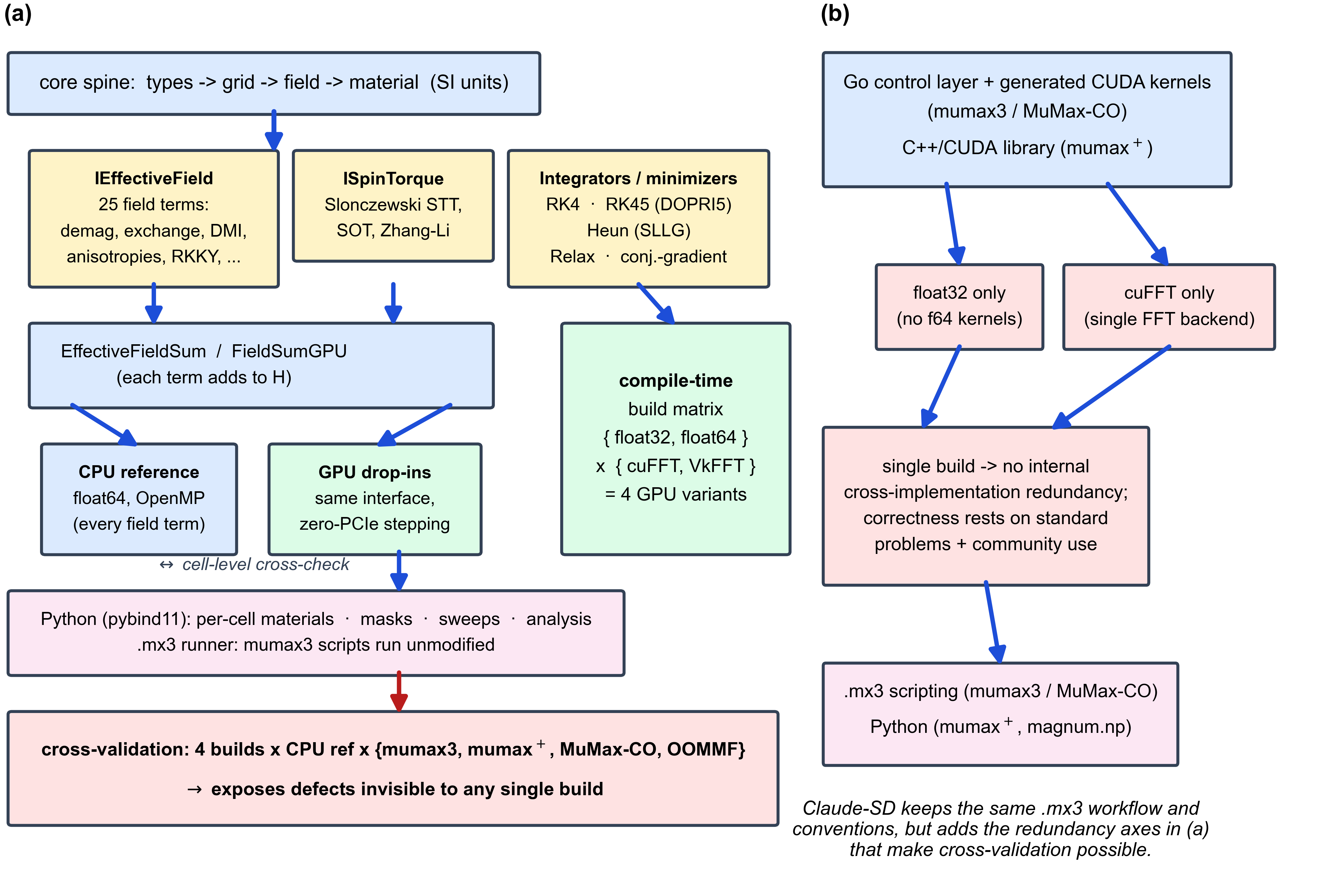
Claude-SD is a C++20 core (Fig. 1) with a narrow IEffectiveField/ISpinTorque/integrator interface: every physics term exists as a float64 CPU reference implementation and, where a GPU build is enabled, a CUDA drop-in behind the same interface. This architecture, to- gether with a Python (pybind11) interface, yields five ways to run the same physics: a CPU library requiring no accelerator at all (validated by the same 236-case Catch2 suite as the GPU path, so every unit test, every µMAG standard problem, and every example notebook runs on a plain laptop), and four GPU build variants selecting float32 or float64 precision and a choice of demagnetization FFT backend: cuFFT, NVIDIA’s proprietary CUDA FFT library, or VkFFT,2 5 an open-source, cross-platform (CUDA/HIP/OpenCL/Level Zero) GPU FFT im- plementation (125 additional GPU-tagged tests). Native effective fields and torques — Zee- man, uniaxial/cubic/surface anisotropy, exchange (Neumann or periodic), open- and periodic- boundary demagnetization, bulk and interfacial DMI, RKKY interlayer coupling, magnetoelas- tic anisotropy, spin–orbit torque, Slonczewski spin-transfer torque, and Zhang–Li torque — are first-class fields with per-cell material control (granular media, composition gradients, multi- 2

layer stacks), rather than user-scripted approximations. Release GPU binaries embed kernels
for compute capabilities 7.5–12.0 (Turing through Blackwell) plus forward-compatible PTX,
and prebuilt Windows packages (CPU and multi-architecture GPU) require no local build at all
(Code availability).

Validation against the µMAG standard problems

Claude-SD reproduces the µMAG standard problems SP#2, SP#4, and SP#5 in their lit- eral geometry and protocol, agreeing with the independent solvers within their mutual spread (Fig. 2, Table 1). For the dynamic switching problem SP#4 (field A), ⟨mx ⟩ at 1 ns is −0.980 (Claude-SD), −0.980 (mumax+ ), −0.969 (mumax3) and −0.984 (OOMMF, CPU double), ver- sus the µMAG reference −0.986 — all within 2%, with the double-precision OOMMF anchor closest. On the SP#1-type flower/vortex crossover example below, Claude-SD and mumax3 agree on the crossover length Lc ≈ 100–120 nm (the precise cross-code-matched sweep in the Showcase section below gives Lc = 115.7 nm to both codes’ agreement). For SP#2, Claude-SD and mumax3 agree on the remanent ⟨mx ⟩ /Ms to ≤ 0.006 at the four cross-checked d/ℓe x points (Supplementary Table S2). SP#5 reproduces the Zhang–Li vortex-core gyration, and a separate idealized-macrospin ferromagnetic-resonance test (no demagnetization, so no finite-size down- shift; NB13, NB48) reproduces the Kittel frequency2 6 to within 0.06% for Claude-SD, mumax3, and mumax+ alike; the confined-island FMR showcase below is a distinct, geometry-resolved test where a downshift from the Kittel value is expected.

Exact agreement with mumax3 under matched conditions, and native .mx3 script execution

Beyond agreement within the standard problems’ mutual spread, Claude-SD was built to match mumax3’s physics conventions exactly wherever a convention is a choice rather than a physical law, so the two codes can be compared under genuinely identical conditions rather than merely similar ones. The interfacial- and bulk-DMI sign, the skyrmion-polarity convention, and the free- boundary condition ∂m/∂n = (D/2A)(ˆz × ˆn) × m at sample edges all follow Rohart–Thiaville2 7 as implemented in mumax3, with no sign remapping in either direction. Run under matched material parameters, cell size, and boundary treatment, the two codes’ relaxed Dzyaloshinskii– Moriya edge-canting profiles agree cell-by-cell to 5×10− 7 (relative), i.e. to single-precision round- off — the floor set by mumax3’s float32 arithmetic for this comparison protocol — not merely “within spread” but numerically the same result. Claude-SD additionally ships micromag.mx3, an interpreter for a practical subset of mu- max3’s own .mx3 scripting language (examples/mx3/, 6 scripts: sp4, disk, regions, relax demo, loop test, and bext ac, plus a further 12 .mx3 scripts in notebooks/mx3/ used for the cross- code showcase comparisons above), so an unmodified community .mx3 script — including the standard-problem script sp4.mx3 used throughout this paper’s benchmarking — runs on Claude- SD’s engine (CPU or GPU, auto-selected) without translation: eng = mm.run mx3("examples/mx3/sp4.mx3", outdir="out") or from the command line, python -m micromag.mx3 examples/mx3/sp4.mx3. Every bench- mark comparison in this paper against mumax3 and MuMax-CO was in fact driven from iden- tical .mx3 scripts (Methods), so the throughput and accuracy numbers reported below already reflect this compatibility rather than a separately-configured native-API equivalent. The inter- preter covers the statements exercised by this paper’s benchmarks and showcase examples and by common community usage, not mumax3’s entire scripting API; the user guide’s mumax3- to-Claude-SD conversion appendix lists supported and unsupported statements and documents the native-API equivalent for any gap. 3

A showcase of representative examples

Beyond the summary statistics above, we walk through seven representative examples in full: each was solved independently with Claude-SD and, where a direct counterpart exists, with a matched mumax3 run on identical geometry, material, and mesh. In every case the two codes agree closely; where a residual difference exists we explain its origin rather than average over it. All examples are distributed as runnable Python notebooks (notebooks/, numbered NBNN ) so a reader can reproduce every figure in this section directly (Code availability). SP#1-type flower/vortex crossover (NB02, NB46). This example asks for the element size at which a thin permalloy square’s ground state switches from a single-domain (“flower” or S-state) texture to a vortex, i.e. the size at which the exchange-energy cost of a vortex core is repaid by the demagnetization-energy saved by flux closure. It uses the same permalloy parameters and the same general element-size-dependent validation goal as µMAG SP#1, but is not literally SP#1’s own hysteresis-loop protocol (Supplementary Information). This is a direct test of the exchange/demagnetization energy balance, independent of dynamics. Fig. 3a sweeps the total energy of both branches over element size L for Claude-SD and a matched mumax3 sweep (identical Ms / Ae x/ α/geometry/mesh): the crossing gives the critical size Lc = 115.7 nm in both codes, to the precision the 20 nm sampling grid resolves. Fig. 3b shows the per-point energy difference is < 1% throughout, with no systematic trend in L — the residual is consistent with ordinary relaxation-tolerance noise, not a physics discrepancy. Fig. 3c,d show the two competing textures directly (S-state and vortex, L = 120 nm, Claude-SD only): the canonical finite-size domain structures the problem is testing for. SP#4 — field-driven switching dynamics (NB01, NB41). Unlike the SP#1-type ex- ample above, SP#4 is a genuinely dynamic benchmark: a reversing field is applied to a thin permalloy strip and the full precessional switching trajectory — not just the final state — must be integrated correctly. Fig. 4a overlays Claude-SD (float64/float32, adaptive RK45) against mumax3 and MuMax-CO across the full 1 ns trajectory; Fig. 4b zooms on the switching event itself (ts w ≈ 175 ps in all solvers). Fig. 4c makes the agreement quantitative: the pointwise difference stays below 1.1 percentage points for the entire trajectory, with the largest deviation — still a small fraction of the trajectory’s full [−1, 1] range — occurring transiently right at the switching event, where the trajectories are most sensitive to last-bit timing differences. This complements the single-endpoint numbers already quoted above (⟨mx ⟩ at 1 ns) with the full time-resolved picture.

Ferromagnetic resonance of a confined island (NB13, NB48). Broadband FMR is a

Ferromagnetic resonance of a confined island (NB13, NB48). Broadband FMR is a standard dynamic-response benchmark distinct from the µMAG suite: a sinc- (Claude-SD) or impulse-excited (mumax3) 80 × 80 × 4 nm permalloy island is left to ring down freely, and the resonance frequency is extracted from the power spectrum (Fig. 5a,b). Because the two codes use different broadband excitation waveforms, their time-domain ring-down envelopes differ (Fig. 5a) — this is expected and does not indicate a physics disagreement, since both waveforms are designed only to excite the same set of normal modes broadband, not to reproduce each other’s transient. The power spectra confirm this: extracted resonance frequencies coincide to within one 0.05 GHz spectral bin (the two peaks fall in the same FFT bin of a 20 ns record; no sub-bin interpolation was applied, Fig. 5c), and both sit below the infinite-film Kittel value2 6 by the same confined-geometry demagnetization downshift. Exchange spin-wave dispersion (NB15). A 1-D permalloy chain excited by a point an- tenna maps out the magnon dispersion relation f (k) (Fig. 6a). Claude-SD and mumax3 ex- tracted peak positions coincide with each other and with the exact finite-difference lattice 4

dispersion at every k (Fig. 6b); both depart from the continuum parabola f ∝ k2 above k ≈ 60 Mrad m− 1 , saturating toward the Brillouin-zone edge. This departure is the expected signature of solving the lattice Laplacian on a finite-difference mesh (which replaces k2 by 4 ∆x2 sin2 (k∆x/2)), not a numerical error in either code — the continuum formula is only valid for k∆x ≪ 1.

Skyrmion D–K phase diagram under matched dynamics (NB21). A seeded Néel

Skyrmion D–K phase diagram under matched dynamics (NB21). A seeded N´eel skyrmion in a Pt/Co film (192 × 192 × 3 nm) is relaxed across a grid of DMI strength D and perpendicular anisotropy Ku , and the relaxed topological charge Q classifies each cell as uni- form, stripe/partial, or skyrmion (Fig. 7), tracing out the phase boundary against the analytic estimate Dc = 4 √ AK/π. When both codes integrate the full Landau–Lifshitz–Gilbert equation (precession and damping) at the same Gilbert damping α = 0.05 for the same physical time (30 ns) — Claude-SD with RK45IntegratorGPU (adaptive DOPRI5), mumax3 with alpha=0.05; Run(30ns) — the seeded skyrmion survives in a band that tracks Dc in both codes, and the cell-by-cell phase classification (uniform/stripe/skyrmion, from |Q|) matches between Claude- SD and mumax3 at 92% of grid points; the residual 8% sits only in the low-Ku / high-D corner, where the ground state is a multi-Q stripe/labyrinth whose exact winding is chaotic and seed- sensitive in any solver. The sign of Q itself is not compared cell-by-cell here: the two codes’ relaxed skyrmions can settle into opposite core polarity from the same nominally-identical seed — an initial-condition/basin choice, not a convention mismatch (Methods documents where sign conventions are matched exactly, e.g. the DMI edge-canting comparison in the Supplementary Information) — so the 92% figure is a sign-insensitive phase-diagram agreement, not a claim that every cell’s signed Q coincides. This is an algorithm-dependent metastability effect: pair- ing Claude-SD’s damped-LLG relaxer or energy minimizer against mumax3’s conjugate-gradient minimizer on this same D–K sweep gives only 53–56% cell-level agreement, because the two re- laxation operators can settle into different metastable (multi-)skyrmion basins near the phase boundary; matching the operator class — both codes integrating the same damped dynamics — raises the agreement to 92%. The lesson generalizes beyond this one example: near a metasta- bility boundary, the relaxation operator is part of the physics being compared, and cross-code agreement should be assessed protocol-by-protocol rather than assumed from a single run.

Replica-batched examples (NB30–32; see Fig. 11, Fig. 12 below). The remaining two

Replica-batched examples (NB30–32; see Fig. 11, Fig. 12 below). The remaining two
examples — thermally-assisted STT switching statistics and the MTJ mesh-convergence study
— exercise the replica-batched engine described below and have no direct mumax3 counterpart,
since batched-ensemble execution is a Claude-SD capability rather than a shared benchmark;
they are validated instead against analytic theory (finite-window N´eel–Brown) and against them-
selves across mesh refinement. We present them together with the replica-batching architecture
in the next subsection rather than duplicating the figures here.
Two further cross-code examples — current-driven domain-wall motion and Walker break-
down, and N´eel-skyrmion DMI edge canting — are presented in the Supplementary Information
with the same level of detail; both show the same pattern of close Claude-SD/mumax3 agreement
once conventions and solver classes are matched.

Capability and performance: a four-solver comparison

We benchmarked Claude-SD against mumax3,1 6 mumax+ (mumaxplus 1.2.1),1 8 and MuMax- CO1 9 — our own previously reported CUDA-Graph-optimized mumax3 fork, included as a per- formance baseline rather than an independent code — on an NVIDIA RTX 5060 Ti (Blackwell, CUDA 13.2). The solvers differ first in capability (Table 1, Fig. 9): the entire mumax3 fam- ily is float32-only and GPU-only, whereas Claude-SD offers float32 and float64 on both CPU and GPU; Claude-SD alone carries two demag FFT backends (cuFFT and VkFFT), native spin–orbit torque,6 per-cell materials, and an automatic integrator selector. For a spintronics 5

workload this capability gap is not cosmetic: chiral textures governed by the Dzyaloshinskii– Moriya interaction,2 7–29 spin–orbit-torque switching,6 and Zhang–Li domain-wall motion3 0, 31 are exactly the problems where topology-sensitive observables benefit from double precision, and where per-cell material control (granular media, composition gradients, multilayer stacks) is required. We therefore compare speed at float32 (the only common precision) and anchor accuracy to Claude-SD’s float64 build. Because the solvers use different-order integrators (RK4 = 4, Dormand–Prince3 2 = 6, Heun = 2 field evaluations per step), the fair throughput metric is milliseconds per field evaluation (Methods). Table 2 and Fig. 8 give the result. Four findings follow. (1) A crossover at ≈0.1–0.5 M cells. Below it, kernel-launch overhead dominates and Claude-SD’s cuFFT float32 build — which captures the per-step kernel sequence as a CUDA Graph3 3 and replays it — is the fastest solver: 5.3× faster than mumax3 and 14× faster than mumax+ at the SP#4 grid, and 2.0×/4.8× at 65 K cells. Above the crossover the comparison becomes cuFFT-bound and the mumax3 family leads, with Claude-SD within 1.57× at 540 K cells and 1.14× at 2.5 M cells. (2) MuMax-CO is the fastest large-grid solver and matches or beats stock mumax3 everywhere: its CUDA-Graph replay removes launch overhead on small grids and reaches parity on large ones (the graph path auto-disables beyond ≈0.8 M cells). On the full SP#4 1-ns adaptive run (integration phase, setup-subtracted), MuMax-CO completes 3.2× faster than stock mumax3 (5.2 s → 1.6 s), with final states agreeing to float32 round-off. (3) mumax+ is the slowest GPU solver on raw throughput at every size; its value lies in extensibility (antiferromagnets, elastodynamics), not speed. (4) The dual-precision advantage is quantitative. Within Claude-SD, float32 is 4–6× faster than float64 at large 3-D sizes on the Blackwell Tensor-Core FFT (e.g. 61.8 → 10.4 ms/step at 540 K cells; 276 → 51 ms/step at 2.5 M), and VkFFT overtakes cuFFT for large float64 trans- forms while losing on small grids — so the two backends are complementary. No competing GPU code exposes a second FFT backend, and none of the codes benchmarked here exposes a precision choice; among GPU micromagnetic codes more broadly, the PyTorch-based mag- num.np2 0 can switch tensor dtype, but without precision-specialized kernels or an alternative FFT backend. The finite-temperature picture mirrors T = 0: with matched Stratonovich–Heun stochastic- LLG integrators3 4, 35 (the only fair SLLG comparison, since MuMax-CO’s graph path is disabled at T > 0 and reduces to mumax3), Claude-SD is 2.1× faster than mumax3 at the SP#4 grid and ≈parity at 0.2 M cells. The comparison is also platform-robust. Claude-SD builds and validates on both Win- dows/MSVC and native Linux/GCC; on a same-host Linux comparison (NVIDIA L4, Ada) the small-grid advantage over mumax3 persists (2.4× at the SP#4 grid, parity at 65 K cells) with the same crossover shape, and it is unchanged when the workload is extended from demag+exchange to a realistic chiral-film field set (interfacial DMI + perpendicular anisotropy). The small-grid win is therefore neither a Windows artifact nor an artifact of a minimal field set. Where each code wins. No single solver dominates on speed (Fig. 8), and on capability only Claude-SD covers every axis (Fig. 9). Claude-SD is preferable for small/2-D dynamics, for any study that needs double-precision reference accuracy or a topology-sensitive observ- able, for development or teaching on a machine without a GPU, and for native custom-torque (SOT/DMI/Zhang–Li) or per-cell-material physics scripted from Python; MuMax-CO/mumax3 are preferable for large float32 production; mumax+ for antiferromagnetic or magnetoelastic problems. That Claude-SD is competitive with — and on small problems faster than — hand- tuned incumbent codes, while adding capabilities they lack, is the central performance result. 6

A replica-batched engine for finite-temperature ensembles

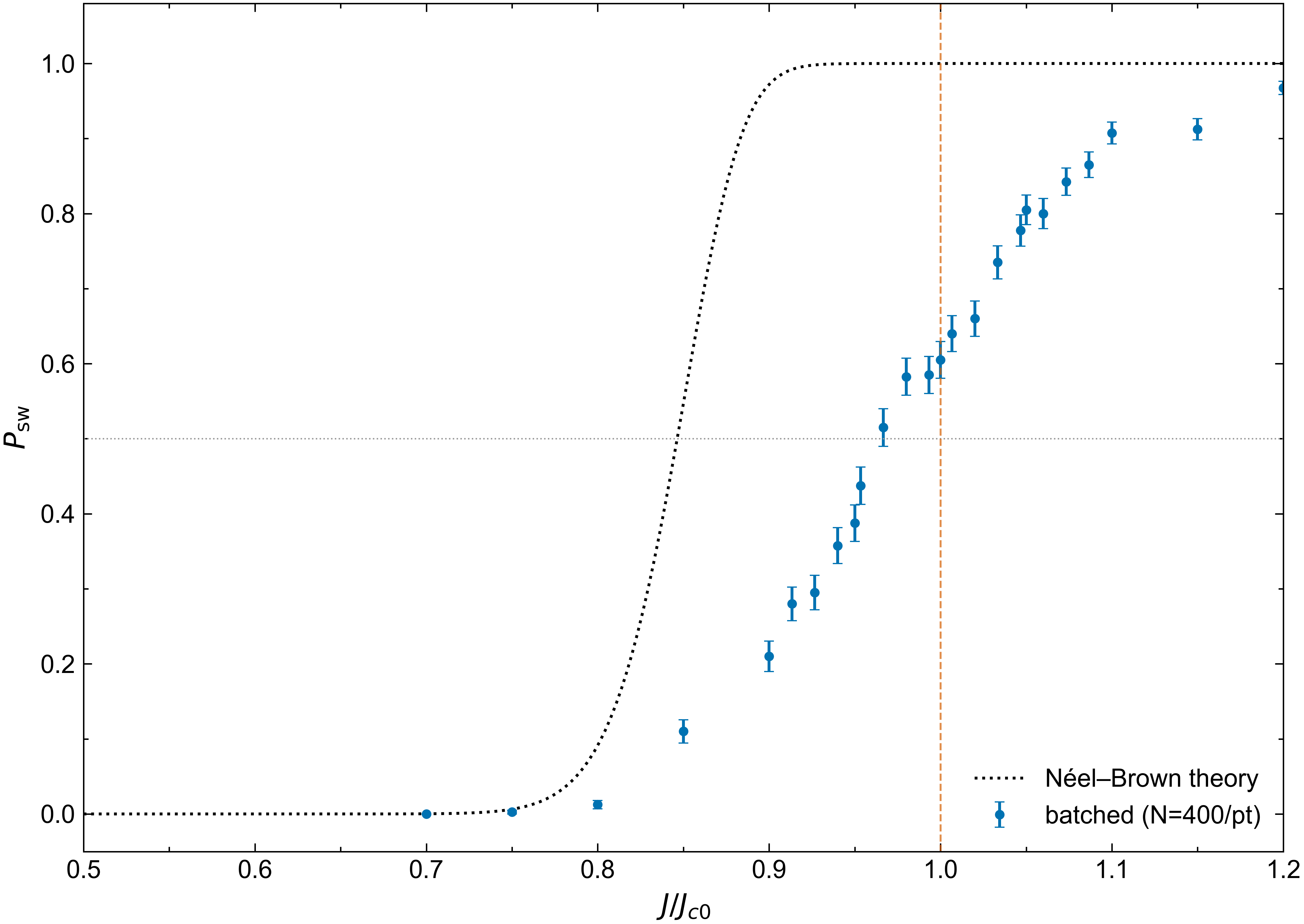
Stochastic switching-probability and bit-error-rate studies — the workload behind thermally- assisted spin-transfer-torque (STT) switching and MRAM reliability estimation — require hun- dreds to thousands of independent finite-temperature trajectories per operating point. Run one trial at a time, each launch leaves the GPU ≈26% utilized (Fig. 10a): the workload is launch- overhead-, not compute-, bound. Claude-SD addresses this with a GPU-resident replica-batching layer (Fig. 10a): a leading replica dimension R is prepended to the magnetization state (replica- outermost, component-major layout, Fig. 10b), and every kernel — rotation-based integration, exchange/uniaxial/Zeeman fields, demagnetization, and thermal noise — advances all R trials in one launch per step, each trial carrying its own current density J and temperature T . Integration uses a norm-exact Depondt–Mertens rotation scheme3 6 (Rodrigues update, |m| = 1 to round-off), verified so that R = 1 reproduces the single-trajectory reference integrator to numerical round-off (max. difference 5.9 × 10− 15 for local fields, 1.3 × 10− 10 for the de- magnetization path, consistent with double-precision FFT round-off). Thermal noise uses a device-side counter-based Philox stream keyed by (seed, replica, step), giving statistically in- dependent, bit-reproducible realizations per trial; the finite-temperature thermal-field variance σ = 2αkB T /(µ2 0M s V γ0 ∆ t) was validated against the parameter-free Langevin equilibrium law ⟨mz ⟩ = L(ξ), ξ = µ0 M s V H/kB T : ⟨mz ⟩ = 0.675 versus L(3) = 0.672. An optional retire/refill mechanism freezes a trial the step it crosses a stop condition (e.g. switched) and reactivates its slot with a fresh noise stream, giving variable-length trials without starving GPU occupancy. Table 3 quantifies the result on a single-cell macrospin (local fields, STT, thermal noise), an 8 × 8 × 1 exchange-and-Zeeman grid, and a 16 × 16 × 1 grid with the full demagnetization path added: this controlled microbenchmark, which isolates pure kernel throughput at matched total work (same physics, same replica count, looped launches vs. one batched launch), gives 55–160×, scaling to 3.7 × 10⁷ replica×step/s at R = 1024. On a full thermally-assisted Slonczewski-STT switching sweep (a Pt/Co-like macrospin, 10,000 replicas × 20,000 steps covering 25 current- density points with 400 trials each), the end-to-end wall time — including the per-trial Python driver and GPU-object setup that the microbenchmark above factors out — drops from ≈2.5 h for a naive per-trial loop to ≈0.6 s batched, a larger ratio than Table 3’s kernel-only figure because the per-trial baseline here also pays non-kernel overhead that the batched path amortizes away entirely; the 55–160× range is the conservative, apples-to-apples number we report as the batching speedup proper. The batched switching probability (Fig. 11) reproduces the sigmoidal shape of the finite-window N´eel–Brown3 4 law with Sun’s antidamping barrier reduction,3 7 Ps w = 1 − exp[−tf0 e − ∆(1−J/Jc 0) 2 ] (clamped at J ≥ Jc 0, with f0 and ∆ fixed independently from the macrospin parameters, no free fit), but the zero-fit-parameter theory curve crosses Ps w = 0.5 at J/Jc 0 ≈ 0.85 while the batched simulation crosses it at J/Jc 0 ≈ 0.97: Sun’s linearized barrier-reduction form is an asymptotic approximation that is known to lose accuracy close to the threshold current itself, where the underlying mean-field treatment of the antidamping torque is least exact, so a threshold offset of this size against the simulated (not merely the analytic) instability point is an expected model limitation rather than a solver discrepancy; the independently measured T = 0 instability current Jc 0 that both curves are normalized by is matched exactly by construction. The speedup makes a discretization-convergence study of the switching threshold practical (Fig. 12): the same 80 × 80 × 1.5 nm CoFeB free layer, meshed at 8 × 8/16 × 16/32 × 32/64 × 64 cells (10/5/2.5/1.25 nm), gives a switching threshold that converges only once the cell size drops below the exchange length ℓe x = 2A/µ0 M 2 s = 4.89 nm: the 16-, 32-, and 64-cell meshes agree on Jc 0 = 0.60 × 101 2 A m− 2 and the fully-switched threshold J(Ps w =1) = 0.63 × 101 2 A m− 2 , while the coarser 8 × 8 mesh (10 nm > ℓe x) under-resolves the reversal and is biased ≈25% high (Jc 0 = 0.75 vs. 0.60 × 101 2 A m− 2 ). Spatially resolving the free layer on the converged 16 × 16 mesh (exchange + demagnetization + Slonczewski STT + thermal noise, versus a coherent whole-layer macrospin at matched T = 0 threshold) also shows a broader, higher-overdrive 7

transition consistent with nucleation-mediated reversal rather than coherent rotation — physics
invisible to the macrospin approximation.

Open availability: examples, notebooks, and documentation

The complete source, unit tests, and benchmark harness are distributed under the GPLv3 license
(Code availability). Beyond the library itself, the repository ships 51 runnable Python example
notebooks spanning every µMAG standard problem, ferromagnetic resonance, spin-wave disper-
sion, domain-wall motion, skyrmion nucleation and phase diagrams, Walker breakdown, spin–
orbit-torque switching, and the finite-temperature replica-batching studies reported above; 9
further API examples (including a ParaView-visualization gallery); and 18 .mx3 scripts runnable
both on mumax3 and on Claude-SD’s own engine (6 general-purpose examples in examples/mx3/
plus 12 used to drive this paper’s cross-code showcase figures, notebooks/mx3/). A 1200-line
user guide documents the full Python API, GPU per-cell field interface, integrator-selection
guidance, and a mumax3-to-Claude-SD conversion appendix, so a reader can reproduce every
figure in this paper, or start a new study, without reading the C++ source.

Discussion

Claude-SD demonstrates that a cross-platform, dual-precision micromagnetic simulator can match the incumbent GPU standard exactly under matched conditions, run its scripts un- modified, and still be faster in the small/2-D regime while adding capabilities the incumbent lacks. Relative to mumax3 — the de facto GPU standard of the spintronics community1 6, 17 — Claude-SD is differentiated on five axes. (i) A CPU build with no GPU requirement: every code we benchmark head-to-head here (mumax3, mumax+ , MuMax-CO) requires an NVIDIA GPU to build or run at all; Claude-SD’s CPU path, validated by the same native-kernel test suite as its GPU path, makes development, teaching, and small-scale production possible on any machine. (ii) Double precision: the mumax3 family is float32-only; Claude-SD’s float64 path en- ables bit-reproducible topological-charge studies, long-time integrations, and energy-landscape resolution that single precision cannot guarantee, at a measured and acceptable cost (float32 remains available and 4–6× faster when precision permits). (iii) Redundant demag backends: cuFFT and VkFFT are complementary in size regime and provide an internal cross-check of the single most error-prone component of any micromagnetic code. (iv) Native spintronics physics: spin–orbit torque, Zhang–Li torque, bulk and interfacial DMI, RKKY interlayer coupling, and magnetoelastic anisotropy are first-class fields rather than user-scripted approximations, with per-cell material control for granular and graded media. (v) A Python-native API with mumax3 compatibility: Claude-SD embeds in the scientific-Python ecosystem (NumPy interchange, and a multiprocessing-safe parameter sweep helper that can distribute independent runs across multi- ple GPUs via per-worker device selection) while also executing mumax3 .mx3 scripts unmodified and matching mumax3 to 5 × 10− 7 under matched conditions, lowering the migration barrier in both directions. mumax3 retains genuine advantages — a decade of community hardening, a large published-results corpus, and the best large-grid float32 FFT throughput — and our data quantify rather than dismiss them. Among the codes not benchmarked here, the PyTorch-based magnum.np2 0 is the closest in capability breadth (including dtype selection and a compara- ble native-physics set) and is uniquely differentiable via autograd for inverse design; its own benchmarks place it within a factor of two of mumax3 at large sizes, while the launch-overhead- dominated small-grid regime — where Claude-SD’s advantage is largest — is a known cost of eager tensor-framework execution. Unlike the mumax3 family, magnum.np is PyTorch-based and so can, like Claude-SD, run its CPU tensor backend without a GPU; Claude-SD’s CPU path differs in being validated by the identical native-kernel test suite used for the GPU path, rather 8

than inheriting CPU support from a general-purpose tensor framework. The two designs are complementary: differentiable simulation versus maximum-throughput, cross-validated native kernels. The replica-batched extension adds a capability none of the benchmarked solvers offers: an entire finite-temperature ensemble advanced in one launch, gated by an R = 1 round-off- identical regression against the single-trajectory integrator on every new kernel. It also surfaced a numerical-accuracy lesson worth stating plainly: because the exchange field scales as 1/dx2 , refining the mesh without shrinking the time step accordingly does not crash — the norm- exact rotation integrator stays stable — it silently suppresses switching and returns a smooth but wrong curve. Finally, because the GPU kernels use no vendor-specific intrinsics, the same backend seam that isolates CUDA from the physics code also isolates it from the vendor: a HIP backend arm compiles and executes through HIP-over-CUDA today, and native AMD/Intel builds are available through collaboration, extending the reach of the codebase beyond the single-vendor GPU ecosystem that constrains mumax3, mumax+ , and MuMax-CO alike. The limitations are bounded honestly. Claude-SD’s damped-LLG relaxer converges more slowly than adaptive minimizers for stiff Dzyaloshinskii–Moriya textures; topological-charge studies near phase boundaries should use the energy minimizer or a larger step budget. The raw-throughput advantage is confined to the small/2-D regime; large float32 production remains the mumax3 family’s domain. The replica-batched demagnetization kernel uses a full-complex (not symmetry-compressed) tensor contraction — simpler and already correct at the single-cell- to-few-thousand-cell scale the batching targets, but not yet the production kernel’s memory- optimized form at large per-replica grids — and no other benchmarked solver here offers a comparable batching feature, so this extension is reported as a capability advance rather than a cross-solver comparison. The .mx3 interpreter covers a practical subset of mumax3’s scripting language (Appendix A of the user guide lists supported and unsupported statements), not its entirety.

Methods

Physics and discretization

Claude-SD integrates dm dt = −γ ′ µ0 (m × H) − γ ′ αµ0 m × (m × H), γ′ = γ0 1 + α2 , (1) on a structured finite-difference grid with x-fastest indexing. Effective-field contributions (each adds to H): Zeeman, uniaxial/cubic/surface anisotropy, six-point Laplacian exchange (Neumann or periodic boundary conditions), open-boundary demagnetization by FFT convolution with the Newell tensor3 8 zero-padded to 2N , periodic-boundary demagnetization by an image-sum kernel, bulk and interfacial DMI, RKKY interlayer exchange, and magnetoelastic anisotropy. The interfacial-DMI sign and skyrmion-polarity conventions follow Rohart–Thiaville2 7 as imple- mented in mumax3, including the free boundary condition ∂m/∂n = (D/2A)(ˆz × ˆn) × m at sample edges (grid and geometry-mask boundaries). One convention difference from mumax3 is documented for reproducibility: the Zhang–Li drift velocity is u = JP µB /(eMs ) (without Thiaville’s 1/(1 + ξ2 ) prefactor3 1 that mumax3 includes). Because Walker breakdown occurs at a fixed dimensionless drift velocity uc set by α and ξ alone, the two conventions map the same physical current J to drift velocities u differing by 1 + ξ2 , so both the sub-Walker drift velocity at a given J and the Walker breakdown current JW itself differ by 1 + ξ2 between the two con- ventions unless matched; an option matches mumax3 exactly when required (used throughout the Zhang–Li showcase and Supplementary comparisons). Spin torques (Slonczewski STT,3 9, 40 spin–orbit torque,6 Zhang–Li3 0 ) are added per integrator stage. Finite-temperature dynamics 9

use the stochastic LLG with a Stratonovich Heun scheme and cuRAND thermal fields,3 4, 35 or the replica-batched Depondt–Mertens scheme (below).

GPU implementation

Effective fields and integrators run entirely on device with no per-step host transfer; a field compositor accumulates contributions either on per-field streams (synchronized between fields) or on a single shared stream (serialized by stream order). Demagnetization uses cuFFT or, optionally, VkFFT;2 5 the CPU reference path uses FFTW,4 1 the long-standing open-source C FFT library on which most CPU micromagnetic codes (including OOMMF) rely. Fixed-step integrators capture the per-step kernel sequence as a CUDA Graph3 3 and replay it. Single and double precision are selected at build time (four preset GPU builds: cuFFT/VkFFT × f32/f64, plus the CPU build). Release binaries embed kernels for compute capabilities 7.5–12.0 (Turing through Blackwell) plus forward-compatible PTX, and the runtime verifies kernel–device compatibility at import. Portability beyond NVIDIA. The GPU layer is written against a thin compile-time back- end seam (runtime, kernel launch, FFT, and RNG), and the kernels use no vendor-specific intrinsics (no warp-shuffle/ballot or texture memory), so a port to other vendors is mechanical rather than structural. A HIP backend arm is provided for AMD (ROCm); its runtime, launch, and RNG paths compile and execute through HIP-over-CUDA (hipcc, HIP PLATFORM=nvidia), validating the seam on a second backend without AMD hardware. An Intel path via SYCL (AdaptiveCpp/DPC++), which additionally runs on CPU, is planned. Native AMD and Intel builds are available through collaboration on request.

Integrators

RK4 (fixed step), RK45 Dormand–Prince (adaptive, first-same-as-last),3 2 Heun (stochastic LLG), a norm-exact Depondt–Mertens rotation scheme3 6 (Rodrigues update; optionally adaptive), damping-only RelaxGPU, and a Barzilai–Borwein/FIRE MinimizeGPU. recommend integrator() selects among them from damping, temperature, goal, and an analytic phase-error estimate, and logs the matched mumax3 SetSolver index so cross-solver runs use equivalent schemes.

Replica batching

The finite-temperature ensemble engine (Results) adds a leading replica dimension R to the Depondt–Mertens integrator: state buffers are laid out replica-outermost and component-major within a replica, local-field, thermal, and demagnetization kernels are re-indexed over R × N threads, and demagnetization batches the forward/inverse FFT over 3R transforms with the Newell kernel tensor3 8 precomputed once and shared across replicas (identical geometry). Cur- rent density J and temperature T are per-replica arrays, giving independent sweep points in a single launch. Thermal noise uses a device-side counter-based Philox generator keyed by (seed, replica-and-cell index, step), reused identically between the predictor and corrector sub-steps (Stratonovich). Every kernel is verified by an R = 1 regression against the single-trajectory DepondtMertensGPU reference trajectory before being accepted.

Benchmark protocol

Throughput was measured by two-run subtraction, [t(N2 ) −t(N1 ) ]/(N2 −N1 ) , to cancel one-time set-up, with size-tiered step counts so the timed difference is several seconds of compute; five measured repeats are reported as median with interquartile range, on an idle RTX 5060 Ti. A cudaDeviceSynchronize precedes every clock stop. Solvers use different-order integrators, so the fair metric is ms per field evaluation (RK4 = 4, Dormand–Prince = 6, Heun = 2 evaluations 10

per step). mumax3 and MuMax-CO were driven from identical .mx3 scripts (Results); mumax+ through its Python TimeSolver; OOMMF via boxsi. The Linux cross-solver comparison used the same protocol on an NVIDIA L4 (Ada, Ubuntu, CUDA 12.4) against the official mumax3 3.12 Linux binary; the mumax3 3.11.1→3.12 version difference was measured on the primary GPU and is ≤ 8% at the smallest grid and ≤ 1% elsewhere. All measurements share one record schema in benchmarks/results/all solvers.json; make report.py regenerates every table and figure from it.

Software availability and reproducibility

The use of AI-assisted coding tools in developing Claude-SD is disclosed in accordance with the
Nature Portfolio policy on large language models: the authors specified the architecture, physics
conventions, and acceptance tests, reviewed every change, and take full responsibility for the
code and this manuscript; no LLM is listed as an author. Build presets, environment, exact
commands, and per-scenario grids are in the Supplementary Information; the full benchmark is
scripted end-to-end and regenerates all tables and figures from a single command.

Data availability

All data supporting the findings of this study — benchmark records (benchmarks/results/
all_solvers.json), µMAG validation outputs, and the scripts that regenerate every table
and figure — are available in the code repository at https://github.com/mirryou-maker/
Claude-SpinDynamics and will be archived on Zenodo with a DOI upon publication.

Code availability

The complete source code of Claude-SD, including the CPU reference implementations, CUDA
kernels, unit tests, and the four-solver benchmark harness, is available under the GPLv3 license
at https://github.com/mirryou-maker/Claude-SpinDynamics (archived on Zenodo; citation
metadata in CITATION.cff). Prebuilt Windows binaries (CPU and multi-architecture GPU
packages, requiring no local build) are provided via GitHub Releases; a 1200-line user guide
(docs/USER GUIDE.md) documents the full API. Beyond the figures shown in this paper and its
Supplementary Information, the same GitHub repository ships substantially more worked exam-
ples than are reproduced here: 51 runnable Python notebooks under notebooks/ (catalogued
in Supplementary Table S8 and in notebooks/GALLERY.md, covering every µMAG standard
problem, FMR, spin-wave dispersion, domain-wall and skyrmion dynamics, Walker breakdown,
spin–orbit-torque switching, and the replica-batched finite-temperature studies), 9 further API
examples, and 18 .mx3 scripts runnable unmodified on either Claude-SD or mumax3 (6 general-
purpose plus 12 driving this paper’s own showcase figures); every one of them regenerates its
own figure(s) against the current build and is a starting point for further exploration.

References

[1] Landau, L. D. & Lifshitz, E. M. On the theory of the dispersion of magnetic permeability in ferromagnetic
bodies. Phys. Z. Sowjetunion 8, 153–169 (1935).
[2] Gilbert, T. L. A phenomenological theory of damping in ferromagnetic materials. IEEE Trans. Magn. 40,
3443–3449 (2004).
[3] Brown, W. F., Jr. Micromagnetics (Interscience, New York, 1963).
[4] Dieny, B. & Chshiev, M. Perpendicular magnetic anisotropy at transition metal/oxide interfaces and appli-
cations. Rev. Mod. Phys. 89, 025008 (2017).
11
[5] Ralph, D. C. & Stiles, M. D. Spin transfer torques. J. Magn. Magn. Mater. 320, 1190–1216 (2008).
[6] Manchon, A. et al. Current-induced spin–orbit torques in ferromagnetic and antiferromagnetic systems. Rev.
Mod. Phys. 91, 035004 (2019).
[7] Parkin, S. S. P., Hayashi, M. & Thomas, L. Magnetic domain-wall racetrack memory. Science 320, 190–194
(2008).
[8] Fert, A., Reyren, N. & Cros, V. Magnetic skyrmions: advances in physics and potential applications. Nat.
Rev. Mater. 2, 17031 (2017).
[9] Mu¨hlbauer, S. et al. Skyrmion lattice in a chiral magnet. Science 323, 915–919 (2009).
[10] Sampaio, J., Cros, V., Rohart, S., Thiaville, A. & Fert, A. Nucleation, stability and current-induced motion
of isolated magnetic skyrmions in nanostructures. Nat. Nanotechnol. 8, 839–844 (2013).
[11] Fidler, J. & Schrefl, T. Micromagnetic modelling — the current state of the art. J. Phys. D: Appl. Phys.
33, R135–R156 (2000).
[12] Miltat, J. E. & Donahue, M. J. Numerical micromagnetics: finite difference methods. In Handbook of
Magnetism and Advanced Magnetic Materials Vol. 2 (Wiley, 2007).
[13] Abert, C. Micromagnetics and spintronics: models and numerical methods. Eur. Phys. J. B 92, 120 (2019).
[14] Leliaert, J. & Mulkers, J. Tomorrow’s micromagnetic simulations. J. Appl. Phys. 125, 180901 (2019).
[15] Donahue, M. J. & Porter, D. G. OOMMF User’s Guide, Version 1.0. Interagency Report NISTIR 6376
(NIST, Gaithersburg, 1999).
[16] Vansteenkiste, A. et al. The design and verification of MuMax3. AIP Adv. 4, 107133 (2014).
3
[17] Leliaert, J. et al. Fast micromagnetic simulations on GPU — recent advances made with mumax . J. Phys.
D: Appl. Phys. 51, 123002 (2018).
+
[18] Moreels, L., Lateur, I., De Gusem, D. et al. mumax : extensible GPU-accelerated micromagnetics and
beyond. npj Comput. Mater. 12, 71 (2026). https://doi.org/10.1038/s41524-025-01893-y
[19] You, C.-Y. Optimization of MuMax3 by using Claude Code: a CUDA-graph-based case study in AI-assisted
performance engineering. J. Magn. 31, 204 (2026). https://doi.org/10.4283/JMAG.2026.31.2.204
[20] Bruckner, F., Koraltan, S., Abert, C. & Suess, D. magnum.np: a PyTorch-based GPU-enhanced finite-
difference micromagnetic simulation framework for high-level development and inverse design. Sci. Rep. 13,
12054 (2023).
[21] Lepadatu, S. Boris computational spintronics — high performance multi-mesh magnetic and spin transport
modeling software. J. Appl. Phys. 128, 243902 (2020).
[22] Bisotti, M.-A. et al. Fidimag — a finite difference atomistic and micromagnetic simulation package. J. Open
Res. Softw. 6, 22 (2018).
[23] Donahue, M. J. & the µMAG group. µMAG Standard Problems. NIST/CTCMS, https://www.ctcms.nist.
gov/~rdm/mumag.org.html.
[24] You, C.-Y. Variance-reduced trajectory unravelings for GPU noisy quantum-circuit simulation: characteri-
zation and a Qiskit-Aer integration gap. Preprint at https://arxiv.org/abs/2607.17678 (2026).
[25] Tolmachev, D. VkFFT — a performant, cross-platform and open-source GPU FFT library. IEEE Access
11, 12039–12058 (2023).
[26] Kittel, C. On the theory of ferromagnetic resonance absorption. Phys. Rev. 73, 155–161 (1948).
[27] Rohart, S. & Thiaville, A. Skyrmion confinement in ultrathin film nanostructures in the presence of
Dzyaloshinskii–Moriya interaction. Phys. Rev. B 88, 184422 (2013).
[28] Dzyaloshinsky, I. A thermodynamic theory of “weak” ferromagnetism of antiferromagnetics. J. Phys. Chem.
Solids 4, 241–255 (1958).
[29] Moriya, T. Anisotropic superexchange interaction and weak ferromagnetism. Phys. Rev. 120, 91–98 (1960).
12

[30] Zhang, S. & Li, Z. Roles of nonequilibrium conduction electrons on the magnetization dynamics of ferro- magnets. Phys. Rev. Lett. 93, 127204 (2004). [31] Thiaville, A., Rohart, S., Ju´e, ´E., Cros, V. & Fert, A. Dynamics of Dzyaloshinskii domain walls in ultrathin magnetic films. Europhys. Lett. 100, 57002 (2012). [32] Dormand, J. R. & Prince, P. J. A family of embedded Runge–Kutta formulae. J. Comput. Appl. Math. 6, 19–26 (1980). [33] NVIDIA Corporation. CUDA C++ Programming Guide — CUDA Graphs; NVIDIA Blackwell Architecture Whitepaper (2024). [34] Brown, W. F., Jr. Thermal fluctuations of a single-domain particle. Phys. Rev. 130, 1677–1686 (1963). [35] Garc´ıa-Palacios, J. L. & L´azaro, F. J. Langevin dynamics study of the dynamical properties of small magnetic particles. Phys. Rev. B 58, 14937–14958 (1998). [36] Depondt, P. & Mertens, F. G. Spin dynamics simulations of soft ferromagnetic nanoparticles at finite temperature. J. Phys.: Condens. Matter 21, 336005 (2009). [37] Sun, J. Z. Spin-current interaction with a monodomain magnetic body: a model study. Phys. Rev. B 62, 570–578 (2000). [38] Newell, A. J., Williams, W. & Dunlop, D. J. A generalization of the demagnetizing tensor for nonuniform magnetization. J. Geophys. Res. 98(B6), 9551–9555 (1993). [39] Slonczewski, J. C. Current-driven excitation of magnetic multilayers. J. Magn. Magn. Mater. 159, L1–L7 (1996). [40] Berger, L. Emission of spin waves by a magnetic multilayer traversed by a current. Phys. Rev. B 54, 9353– 9358 (1996). [41] Frigo, M. & Johnson, S. G. The design and implementation of FFTW3. Proc. IEEE 93, 216–231 (2005).

Acknowledgements

This work was supported by the National Research Foundation of Korea (NRF) (No. RS-2026-
25502724) and the Strategic Research Program under the DGIST R&D Program (26-SR-01) of
the Ministry of Science, ICT, and Future Planning.

Author contributions

C.-Y.Y. conceived the study, directed development, designed the validation and benchmark
protocols, analyzed the data, and wrote the manuscript. J.C. contributed to validation and
reviewed the manuscript.

Competing interests

The authors declare no competing interests.

Ethics declarations

Ethics approval and consent to participate. Not applicable: this study did not involve
human participants, human data or tissue, or animal subjects.
Consent for publication. Not applicable.
13

Materials availability

This study did not generate physical materials. All computational materials — source code,
build configurations, and benchmark/validation data — are covered under Code availability
and Data availability above.

Supplementary information

Supplementary Information is included as an ancillary file with this arXiv submission, and is also
available with the published version of this article, including extended benchmark methodology,
full standard-problem protocol details, the complete precision/race-condition study, the AI-agent
development protocol, additional cross-code validation figures (Walker breakdown and DMI edge
canting), and the full example-notebook catalog.
14

Tables

Table 1: Solver capability. Claude-SD alone offers a CPU build requiring no GPU, dual precision, a second FFT backend, natively implemented spin–orbit torque and per-cell materials, and an automatic integrator selector. Scripting: Py = Python API, C++ = native library, mx3 = mumax3 .mx3 interpreter. † mumax3 has no first-class RKKY field; inter-layer exchange coupling is instead scripted via its ext InterExchange/ext ScaleExchange region-rescaling mechanism. Runs w/o GPU Precision Demag FFT Native Scripting

Runs w/o GPU Precision Demag FFT Native SOT/DMI/RKKY/ME Scripting Claude-SD yes (CPU) f32 + f64 cuFFT & VkFFT all native + per- cell + auto-select Py + C++ + mx3 mumax3 no f32 cuFFT DMI; STT via Slon- czewski, no native SOT; no RKKY† .mx3 MuMax-CO no f32 cuFFT = mumax3 (+ CUDA-Graph path) .mx3 mumax+ no f32 cuFFT DMI, AFM, elas- todynamics Py Table 2: Throughput, ms per field evaluation (float32, T = 0; lower is better; median of five repeats). CS = Claude-SD. Bold marks the fastest solver per row. Scenario cells dim CS cuFFT f32 CS VkFFT f32 mumax3 MuMax-CO mumax+ SP#4 2-D 10 K 2D 0.042 0.157 0.223 0.211 0.595 pow-2 3-D 65 K 3D 0.155 0.295 0.305 0.290 0.739 medium 3-D 540 K 3D 2.610 2.777 1.708 1.663 3.302 large 3-D 2.5 M 3D 12.72 13.16 11.28 11.13 18.87

SP#4 2-D 10 K 2D 0.042 0.157 0.223 0.211 0.595 pow-2 3-D 65 K 3D 0.155 0.295 0.305 0.290 0.739 medium 3-D 540 K 3D 2.610 2.777 1.708 1.663 3.302 large 3-D 2.5 M 3D 12.72 13.16 11.28 11.13 18.87 Table 3: Replica-batching throughput (Claude-SD only; no comparable feature exists in mumax3, mumax+ , or MuMax-CO). Speedup is one batched launch of R replicas versus R sequential per-trial launches, at matched total work; R = 1 reproduces the single-trajectory reference trajectory to round-off in every case (Methods). Physics Grid R Speedup vs. loop Throughput at R=1024 Macrospin (local fields + STT + ther- mal) 1 × 1 × 1 256 158.7× 3.7 × 107 replica·step/s Multi-cell (exchange + uniaxial + Zee- man) 8 × 8 × 1 64 59.8× 1.4 × 108 cell·step/s (R=256) Multi-cell + demagnetization 16 × 16 × 1 64 55.4× 8.9 × 107 cell·step/s (R=256) 15

Figure legends

Figure 1: Claude-SD code architecture versus the incumbent GPU-only design.

Figure 1: Claude-SD code architecture versus the incumbent GPU-only design. (a) Claude-SD: a value-type core spine feeds narrow IEffectiveField/ISpinTorque/integrator interfaces; every term exists as a float64 CPU reference and, where enabled, a GPU drop-in be- hind the same interface, compiling into a CPU build plus a {float32, float64}×{cuFFT, VkFFT} GPU build matrix. (b) The monolithic float32/cuFFT/GPU-only mumax3 family, shown for contrast; the .mx3 runner keeps the incumbent scripting workflow unchanged on Claude-SD. 16

Figure 2: µMAG standard-problem validation (SP#2, SP#4, SP#5) and an SP#1-

Figure 2: µMAG standard-problem validation (SP#2, SP#4, SP#5) and an SP#1- type flower/vortex crossover (Claude-SD, float64). Claude-SD’s own solution for all four panels; its agreement with mumax3, mumax+ , MuMax-CO and the double-precision OOMMF anchor within their mutual spread is quantified numerically in the main text (Results) and the Supplementary Information’s standard-problem tables, rather than overlaid on these panels. (a) SP#1-type: S-state/vortex energy crossing at Lc (not literally µMAG SP#1’s hysteresis- loop protocol; Supplementary Information). (b) SP#2: remanent ⟨mx ⟩ , ⟨my ⟩ versus d/ℓe x. (c) SP#4 field A: ⟨m⟩(t), with the µMAG reference ⟨mx ⟩ (1 ns) = −0.986 dotted (Claude-SD value in text). (d) SP#5: Zhang–Li vortex-core trajectory over 8 ns. 17

Figure 3: SP#1-type showcase: flower/vortex crossover, Claude-SD vs mumax3. (a) Total energy of the S-state and vortex branches vs. element size L (t = 10 nm) for Claude- SD and a matched mumax3 sweep (identical Ms / Ae x/ α/geometry/mesh): the crossing gives Lc = 115.7 nm in both codes. (b) Energy difference (EC laude−SD − Em x3) /Em x3 vs. L: < 1% at every point for both branches. (c,d) Claude-SD-only domain maps at L = 120 nm: S-state (E = 4.13 aJ) and vortex (E = 4.04 aJ), the canonical finite-size textures the crossing in (a) separates.

Figure 4: SP#4 showcase: field-driven switching dynamics, Claude-SD vs mumax3
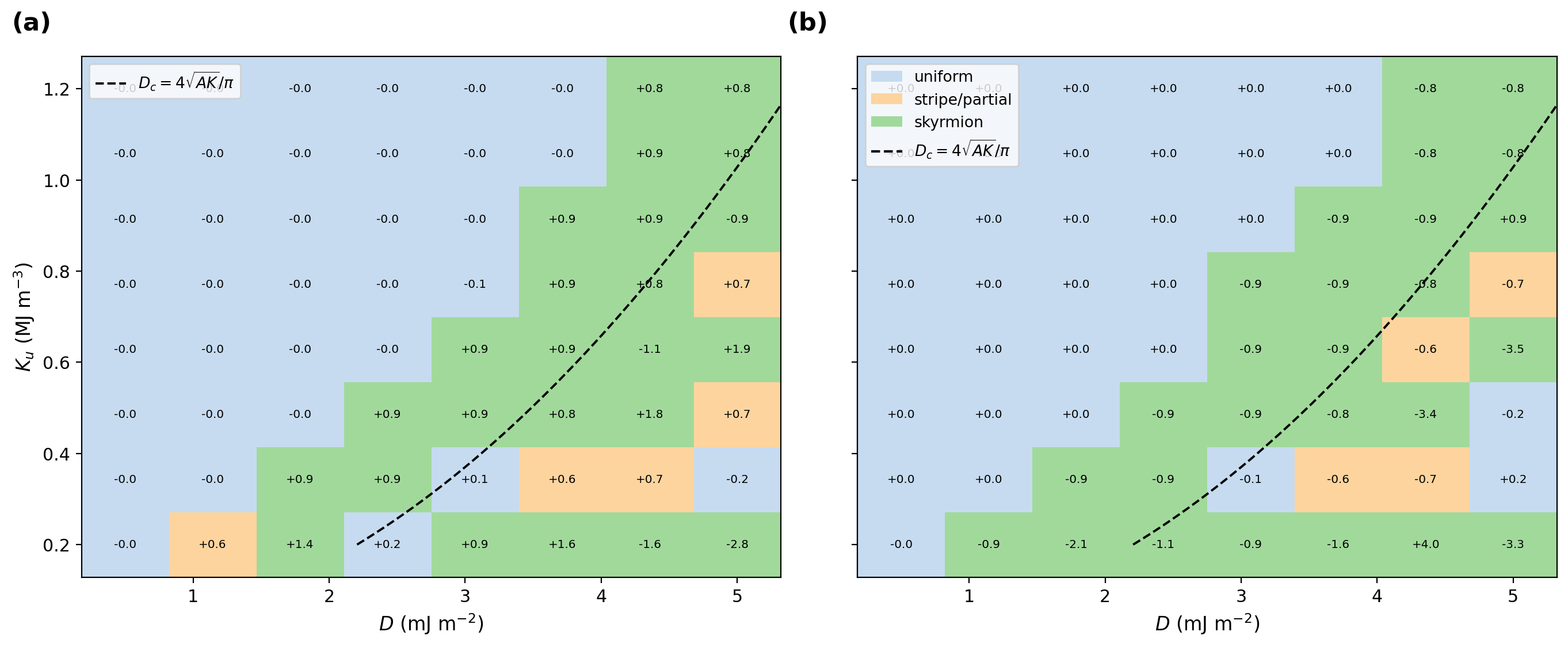
Figure 4: SP#4 showcase: field-driven switching dynamics, Claude-SD vs mumax3 vs MuMax-CO. (a) ⟨mx ⟩ (t) over the full 1 ns reversal of the 500 × 125 × 3 nm permalloy strip, Claude-SD float64/float32 (adaptive RK45) vs. mumax3 vs. MuMax-CO, with the µMAG consensus ⟨mx ⟩ (1 ns) = −0.9862 (dotted). (b) Zoom on the switching region; all solvers cross ⟨mx ⟩ = 0 at ts w ≈ 175 ps. (c) Pointwise difference ⟨mx ⟩ C laude−SD −⟨mx ⟩ m umax3 (and vs. MuMax- CO): < 1.1 percentage points throughout, largest at the switching transient. 18

Figure 5: FMR showcase: broadband ferromagnetic resonance of an 80 × 80 × 4 nm permalloy island, Claude-SD vs a matched mumax3 run. (a) ⟨mz ⟩(t) ring-down

permalloy island, Claude-SD vs a matched mumax3 run. (a) ⟨mz ⟩(t) ring-down (Bb ias = 20 mT in-plane) — Claude-SD driven by a continuous sinc-field pulse, mumax3 by a brief broadband kick on the identical geometry/material; the excitation waveforms differ, so the time-domain envelopes differ, but both probe the same normal mode. (b) Power spectrum (20 ns record, ∆f = 0.05 GHz): the island’s quasi-uniform mode lies below the infinite-film Kit- tel value2 6 because of finite-size in-plane demagnetization, reproduced identically by both codes. (c) Extracted resonance frequencies: Claude-SD and mumax3 coincide to within one 0.05 GHz spectral bin.

Figure 6: Spin-wave dispersion showcase: Claude-SD vs mumax3 vs lattice theory.

Figure 6: Spin-wave dispersion showcase: Claude-SD vs mumax3 vs lattice theory. 1-D permalloy chain (200 × 1 × 1, ∆x = 20 nm, B0 = 0.1 T, demag off; ∆x exceeds the permalloy exchange length ℓe x ≈ 5.7 nm by design, since this test targets the discrete lattice Laplacian’s own dispersion, not continuum-limit micromagnetic accuracy, and demagnetization is switched off so both codes solve the identical exchange-only dispersion relation exactly). (a) Claude-SD S(k, f ) map with the continuum parabola f = γ0 2π (B0 + 2A Ms k2 ) (white) and the exact finite-difference lattice dispersion f = γ0 2π B0 + 2A Ms 4 ∆x2 sin2 k∆x 2 (cyan). (b) Extracted peak positions — Claude- SD and mumax3 (identical chain, point-antenna excitation) coincide with each other and with the lattice curve at every k; both depart from the continuum parabola above k ≈ 60 Mrad m− 1 , the expected finite-difference-lattice signature, not a code discrepancy. 19

Figure 7: Skyrmion D–K phase diagram under matched dynamics, Claude-SD vs mu-
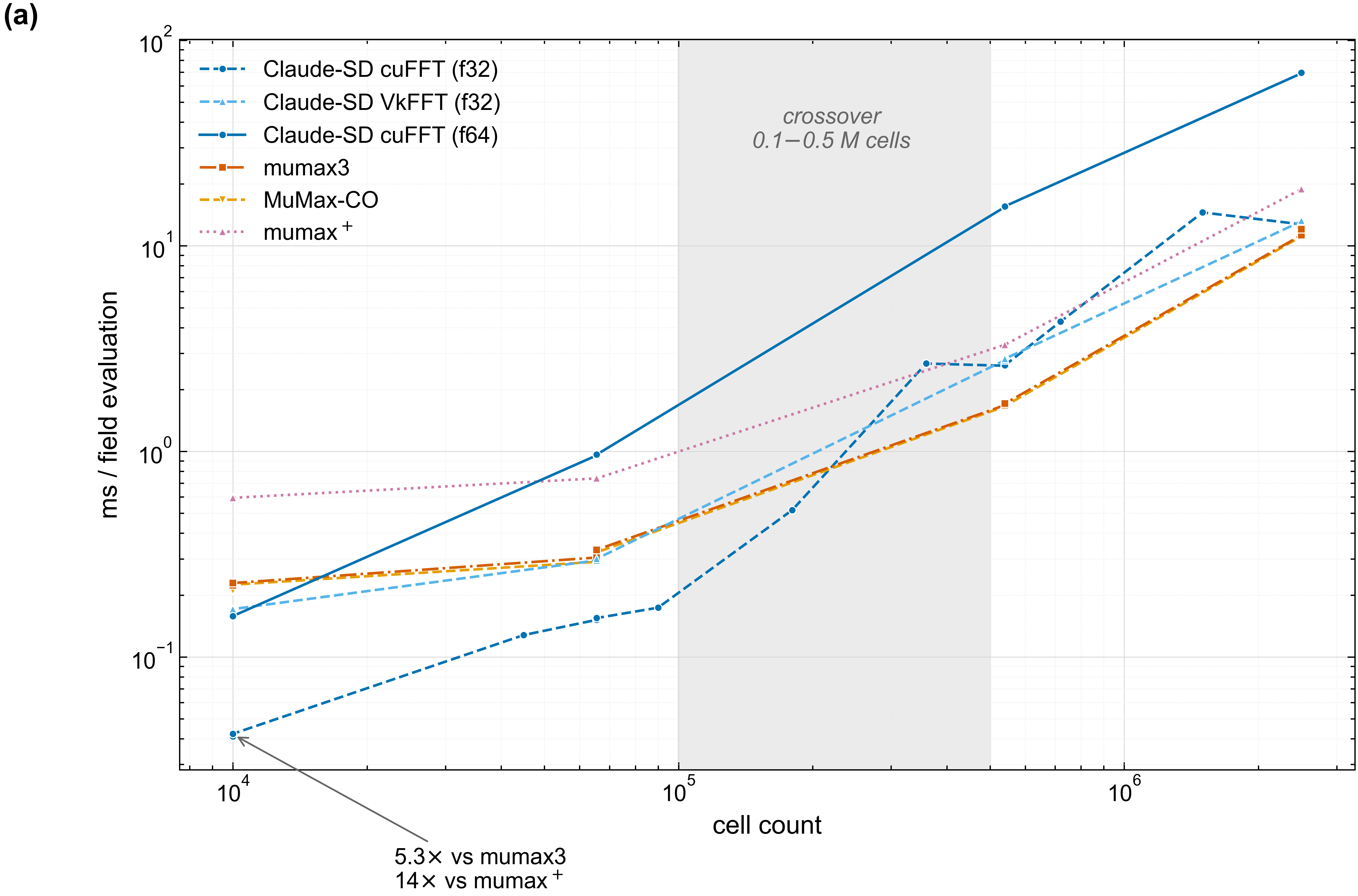
Figure 7: Skyrmion D–K phase diagram under matched dynamics, Claude-SD vs mu- max3: 92% cell-level agreement. Pt/Co film (192 × 192 × 3 nm), identical N´eel-skyrmion seed, both codes integrating the full Landau–Lifshitz–Gilbert equation (precession and damp- ing) at the same Gilbert damping α = 0.05 for the same physical time (30 ns) — Claude-SD with RK45IntegratorGPU (adaptive DOPRI5) (a), mumax3 with alpha=0.05; Run(30ns) (b). Cells show the relaxed topological charge Q (sign as computed by each code), classified uni- form/stripe/skyrmion by |Q|, with the analytic boundary Dc = 4 √ AK/π overlaid. The seeded skyrmion survives in a band that tracks Dc in both codes, and the cell-by-cell phase classifi- cation matches between Claude-SD and mumax3 at 92% of grid points; the residual 8% sits only in the low-Ku / high-D corner, where the ground state is a multi-Q stripe/labyrinth whose exact winding is chaotic and seed-sensitive in any solver. This 92% is sign-insensitive (uni- form/stripe/skyrmion classification only): the relaxed core polarity itself can differ between the two codes at a given grid point, an initial-condition/basin effect rather than a sign-convention mismatch (main text). 20
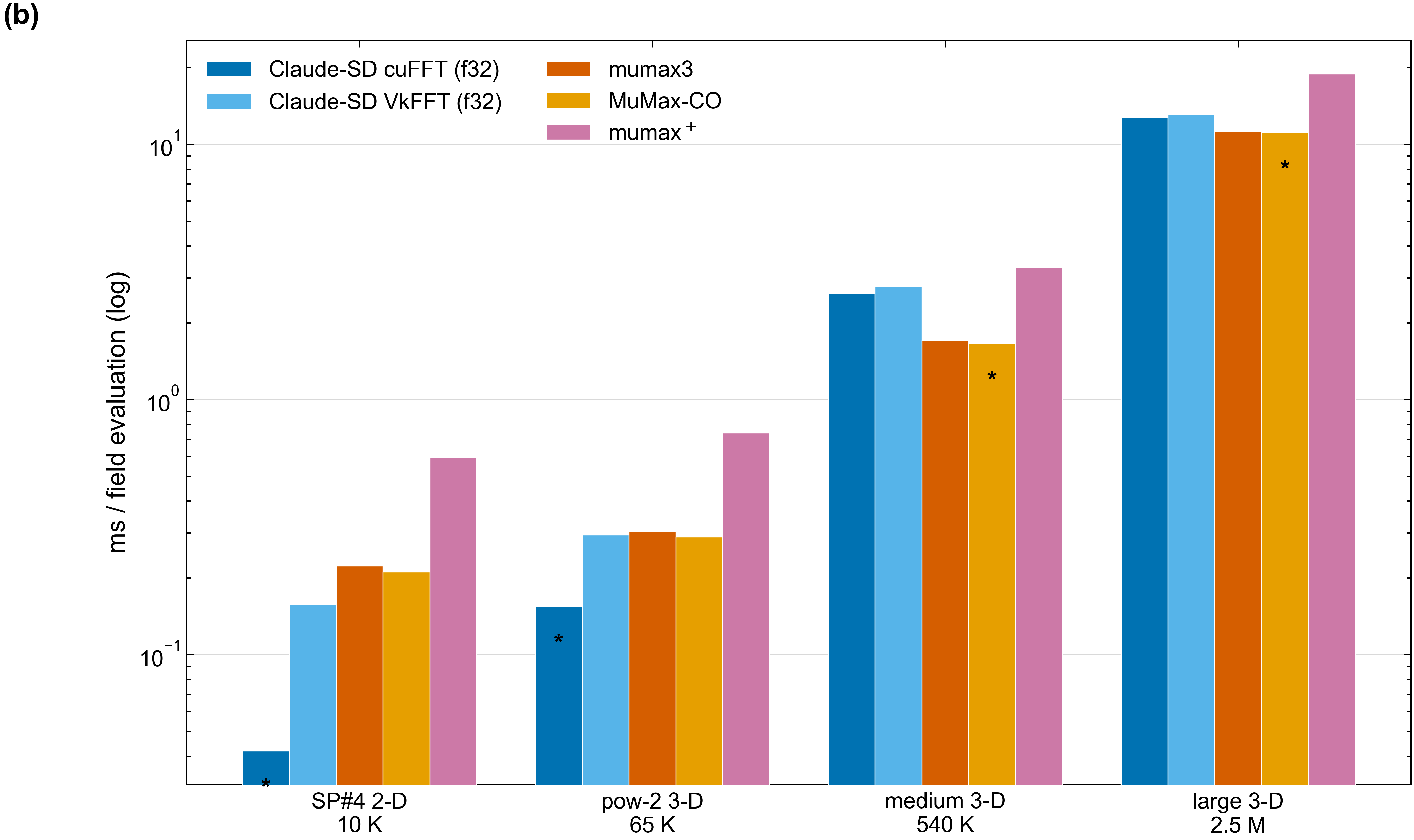
Figure 8: Four-solver throughput. (a) ms per field evaluation versus cell count: Claude-SD float32 leads below the ≈0.1–0.5 M-cell crossover; the mumax3 family leads above it. (b) Per- scenario bars for the four benchmark grids (Table 2); the asterisk above a bar marks the fastest solver for that scenario. 21

Figure 9: Solver capability matrix. Only Claude-SD covers every axis: a CPU build requiring no GPU, double precision, a second FFT backend (VkFFT), native SOT, RKKY, magnetoelastic coupling, per-cell materials, and automatic integrator selection. Figure 10: The replica-batching execution model. (a) A per-trial loop issues R separate kernel launches per step, one host round-trip each, leaving the GPU ≈26% utilized; replica- batching instead appends a replica dimension so rotation update, all fields, and thermal noise for all R trials advance together in a single kernel launch per step, at ≫90% utilization and 55–160× the per-trial-loop throughput at matched R. R=1 reproduces the single-trajectory reference integrator to round-off, so batching changes only performance, not physics. (b) The corresponding GPU state layout: replica-outermost, component-major within each replica (m[r · 3N + c · N + idx]), so one kernel launch indexes all R × 3N entries with no per-replica PCIe transfer after the initial upload. 22

Figure 11: Replica-batched thermally-assisted STT switching. Switching probability of a Pt/Co macrospin (10 nm cell, thermal stability ∆3 00K = KV /kB T = 121, instability threshold Jc 0 = 2.60×101 2 A m− 2 ) versus normalized current J/Jc 0: 10,000 GPU replicas (400 trials/point, 25 points), advanced by one kernel launch per step, complete the full sweep in ≈0.6 s versus ≈2.5 h for a naive per-trial loop (end-to-end wall time, including per-trial driver overhead ab- sorbed by batching; Table 3’s matched-work kernel-only comparison gives the more conservative 55–160×). The batched result reproduces the sigmoidal shape of the finite-window N´eel–Brown3 4 law with Sun’s barrier reduction3 7 (dashed, zero free parameters) but crosses Ps w = 0.5 at a ≈14% higher J/Jc 0 than the analytic curve, an expected limitation of Sun’s linearized threshold approximation (main text); the T = 0 threshold Jc 0 is measured independently from a small-tilt seed (main text).

Figure 12: Mesh convergence of the STT switching threshold, enabled by replica-

Figure 12: Mesh convergence of the STT switching threshold, enabled by replica- batching throughput. The same 80 × 80 × 1.5 nm CoFeB free layer discretized on 8/16/32/64- cell meshes (10/5/2.5/1.25 nm cells); the absolute current is raised until Ps w = 1 (300 K, 2 ns; every trial a batched replica). (a) The threshold converges once the cell size drops below the exchange length ℓe x = 4.89 nm — the 16/32/64 meshes coincide while the 8 × 8 mesh (10 nm > ℓe x) under-resolves the reversal and is biased high. (b) Normalizing each curve by its own Jc 0 nearly collapses them, showing the mesh effect is almost entirely in the absolute threshold, not the transition shape. 23