⬇ Download Markdown · ⬇ Download LaTeX · ⬇ original · view original · CSV: table 1 , table 2
IRSSG: An Open-Source Software Package for Spin Space Groups
Sheng Zhang, 1 , 2, ∗ Ziyin Song, 1 , 2, ∗ Zhong Fang, 1 , 2 Hongming Weng, 1 , 3 and Zhijun Wang 1 , 3, †
arXiv:2511.21821v2 [cond-mat.mtrl-sci] 20 May 2026
1 Beijing National Laboratory for Condensed Matter Physics, and Institute of Physics, Chinese Academy of Sciences, Beijing 100190, China
2 University of Chinese Academy of Sciences, Beijing 100049, China 3 Condensed Matter Physics Data Center, Chinese Academy of Sciences, Beijing 100190, China
C ondensed Matter Physics Data Center, Chinese Academy of Sciences, Beijing 100190, China (Dated: May 21, 2026) We present an open-source software package IRSSG for investigating magnetic systems with spin space groups (SSGs). The package works within the density functional theory (DFT) framework and requires wavefunctions from DFT codes, such as VASP, Quantum ESPRESSO, as well as any other code that has an interface to Wannier90. We introduce a set of compact SSG international symbols by combining non-crystallographic point groups with the 230 crystallographic space groups. The program first identifies all SSG operations and determines the SSG international symbol for a given magnetic system. It then generates the SSG character tables of little groups at any k point. Finally, it computes the traces of matrix representations of SSG operations and assigns irreducible corepresentation labels to magnetic energy bands. The program is not only timely but also essential for advancing research on the study of magnons, altermagnetism, magnetic topology, and novel high-degeneracy excitations in SSG systems.
Program summary Program title: IRSSG
Program title: IRSSG CPC Library link to program files: https://doi.org/10.17632/sjyxmpr9gw.1 Licensing provisions: GNU General Public Licence 3.0 Programming language: Python 3, Fortran 90 Nature of problem: Determining the irreducible corepresentations of band structures under spin space groups (SSGs) is particularly valuable for band-character assignment, connectivity analysis, and topology diagnostics in SSG systems. Solution method: The program identifies all SSG operations and determines the corresponding SSG international symbol. It constructs the k -little-group character tables using the Hamiltonian method, and determines the band irreducible corepresentations by comparing the traces of matrix representations of SSG operations acting on DFT wavefunctions or Wannier tight-binding states. DOI: 10.1016/j.cpc.2026.110190
I. INTRODUCTION
Symmetry plays a fundamental role in condensed matter and materials physics by facilitating the prediction of emergent phenomena and material properties, such as ferroelectricity [ 1 – 3 ], phonons [ 4 – 6 ], topological insulators [ 7 – 10 ], and superconductivity [ 11 – 13 ]. Symmetry also provides powerful constraints that significantly simplify otherwise complex many-body problems. For crystals, the symmetries are categorized into 230 crystallographic space groups (CSGs). In magnetic materials, a variety of spin configurations ( e.g. , ferromagnetic, antiferromagnetic, and helical orders) can emerge. To describe such materials in the presence of spin–orbit coupling (SOC), the time-reversal oper- ation T is combined with the 230 CSGs, resulting in 1651 Shubnikov magnetic space groups (MSGs) [ 14 ]. However, in the weak-SOC regime relevant for many magnetic materials and magnons, the spin and lattice degrees of freedom largely decouple, leading to a richer symmetry structure beyond MSGs. Therefore, Brinkman and Elliott introduced the concept of spin space groups (SSGs), where spin and lattice operations are treated individually, without be- ing rigidly tied [ 15 ]. Later, Litvin provided a mathematically rigorous formulation of SSGs [ 16 ] and systematically enumerated their corresponding spin point groups [ 17 ]. In this SOC-free setting, Liu et al. provided a modern formu- lation of spin-group symmetry and clarified its implications for condensed-matter Hamiltonians and applications [ 18 ]. Building on these developments, several recent works have achieved a comprehensive enumeration and classification of SSGs [ 19 – 21 ]. The SSGs are now widely used in the analysis of topological electronic bands, magnon spectra [ 22 , 23 ], supercon- ducting order parameters [ 24 ], altermagnetism [ 25 , 26 ], anomalous Hall responses [ 27 ], etc. Jiang et al. systematically ∗ These authors contributed equally to this work. † Electronic address: [email protected] ; The codes are available in the public repository: https://github.com/zjwang11/IRSSG/ .
2 enumerated all such SSGs, including 1421 collinear groups, 24,788 coplanar noncollinear groups, and 157,289 non- coplanar groups, in which the magnetic primitive cell is at most twelve times the atomic primitive cell [21]. In addition, Chen et al. proposed an international symbol for SSGs. However, these Chen-Liu symbols can be rather involved because they are constructed within a classification scheme that divides SSGs into three types [20]. Later, they further developed an oriented international notation for SSGs, which explicitly encodes the absolute orientation of magnetic moments [28]. Nonetheless, since this notation is also based on the same three-type classification, its explicit form may vary substantially from case to case, leading to additional complexity. For nonmagnetic and magnetic topological materials, the program IRVSP/IR2TB [29] represents the first compu- tational tool capable of determining irreducible (co)representations [(co)irreps] and uncovering the band topology of electronic band structures computed using density functional theory (DFT) codes such as VASP [30, 31], Quantum ESPRESSO [32, 33], as well as any other code that has an interface to Wannier90 [34, 35]. It can generate the input files needed to calculate elementary band representations and symmetry-based indicators via the TopMat [36] or Check Topological Mat server [37]. Within this band-representation framework, methods have also been developed to diagnose unconventional materials with obstructed atomic limit via the BRdecomp server [38]. In this work, we de- velop IRSSG to obtain the SSG coirreps of the band structures of magnetic materials with arbitrary SSG symmetries for the first time. IRSSG identifies all SSG operations and determines the SSG number and international symbol. Meanwhile, we introduce a set of compact SSG international symbols by combining non-crystallographic point groups with the 230 crystallographic space groups. The paper is structured as follows. In Section II, we present the methods implemented in our program, including the basic concepts of SSGs as well as the method to construct coirreps based on SSG operations and to obtain matrix representations of materials. In Section III, the general workflow of the IRSSG code is described in detail. The capabilities of IRSSG are described in Section IV. In Section V, we introduce the installation steps and usage of the program. Some typical examples are shown in Section VI. In Appendix A, we provide a side-by-side comparison between the symbols output by IRSSG and Chen-Liu symbols.
II. BASIC CONCEPTS OF SPIN SPACE GROUPS AND COIRREPS
A. Spin space groups and international symbols
Given a magnetic crystal structure with atoms { s i , r i , X i } , SSG operations are defined as G = {O α ≡ {U α | |R α | v α } |U α s i = s j , R α r i + v α = r j , X i = X j }, U α ∈ O (3) , det( U α ) = +1 , O α is unitary without T , − 1 , O α is anti-unitary with T , R α ∈ O (3) , det( R α ) = +1 , R α is a proper rotation without I, − 1 , R α is an improper rotation with I. (1) Here s i , r i , and X i are the magnetic moment, position, and element type of the i th atom, respectively. An SSG operation is denoted as O α = {U α | |R α | v α } , consisting of a spin part U α and a lattice part {R α | v α } . The time-reversal ( T ) symmetry reverses the spin direction and acts as an ‘inversion’ symmetry in spin space. Therefore, det( U α ) = − 1 indicates the presence of T , being an anti-unitary symmetry. The det( R α ) = − 1 indicates the presence of inversion ( I ), resulting in an improper rotation. In an SSG, the spin rotation U α and lattice rotation R α are O (3) matrices and independent. In a sense, the 230 CSGs and 1651 MSGs are special cases of SSGs. Explicitly, a CSG is an SSG with U α = E for all O α ∈ G , while an MSG is an SSG with U α = ±R α (sharing the same proper rotation) for all O α ∈ G . Therefore, although IRSSG is developed for SSGs, it also works for the 230 CSGs and 1651 MSGs. In general, a special subgroup of G is defined as the spin-only group, S 0 ≡ {O α ∈ G|{R α | v α } = {E| 0 }}, G 0 = G/S 0 , G = S 0 × G 0 (2) which contains the SSG operations whose lattice part is the identity. Since the coset representatives of G/S 0 form a group ( G 0 ) , G can be expressed as a direct product of S 0 and G 0 . According to the magnetic configuration, SSGs can be classified into three types: collinear (I), coplanar (II) and noncoplanar (III), each corresponding to a specific spin-only group, as shown in Table I . We now introduce two groups derived from G 0 : the spin part group P and the lattice part group H , P ≡ {U α | ∀O α ∈ G 0 } , H ≡ {{R α | v α } | ∀O α ∈ G 0 } . (3)
3 Table I: Spin space groups and international symbols. The non-crystallographic point group P (in Sch¨onflies notation) is the group formed by the spin parts of the elements of G 0 in Eq. ( 3 ). Its elements are listed as α , β , γ , δ , et al. , denoted in Hermann–Mauguin notation. The crystallographic space group H is the group formed by the lattice parts of G 0 in Eq. ( 3 ), whose international notation is Xxyz. X stands for the Bravais-lattice type and x / y / z are the Hermann–Mauguin symbols of the rotational generators. A compact SSG international symbol can be expressed in the form of X α ,β,γ x δ y ϵ z η ( P I / II / III ). Spin space group G and international symbol X α ,β,γ x δ y ϵ z η ( P I / II / III ) ( G = S 0 × G 0 ) Magnetic Configuration Spin-only group S 0 Group G 0 P (spin part) H (lattice part) G 0 generators ( P ≡ {α, β, γ, δ, · · · } ) X : a 1 , a 2 , a 3 x / y / z X α ,β,γ x δ I: Collinear {{C ∞ z ||E| 0 }, {M x C ∞ z ||E| 0 }} C 1 , C i P: 100 , 010 , 001 C: 1 2 1 2 0 , ¯ 1 2 1 2 0 , 001 I: ¯ 1 2 1 2 1 2 , 1 2 ¯ 1 2 1 2 , 1 2 1 2 ¯ 1 2 A: 100 , 0 1 2 ¯ 1 2 , 0 ¯ 1 2 1 2 F: 0 1 2 1 2 , 1 2 0 1 2 , 1 2 1 2 0 R: 2 3 ¯ 1 3 ¯ 1 3 , 1 3 1 3 ¯ 2 3 , 1 3 1 3 1 3 1, ¯ 1, 2, 2 1 , 3, ¯ 3, 3 1 , 3 2 , 4, ¯ 4, 4 1 , 4 2 , 4 3 , 6, ¯ 6, 6 1 , 6 2 , 6 3 , 6 4 , 6 5 , a , b , c , d , e , m , n {α||E| a 1 } , {β||E| a 2 } , {γ||E| a 3 } {δ|| x } II: Coplanar {{E||E| 0 }, {M z ||E| 0 }} C 1 , C i , C s , C n , C n v ( n ≥ 2) III: Noncoplanar {{E||E| 0 }} C 1 , C i , C s , C n , C n v , C n h , S 2 n , D n , D n h , D n d , T , T h , T d , O , O h , I , I h Clearly, P belongs to a non-crystallographic point group (NPG), while H belongs to a CSG. Thus, any SSG operation of G 0 can be expressed by an element (x) of H , with a superscript element ( δ ) of P ( i.e. , x δ ≡ {δ|| x } ). Based on the above analysis of the SSG group structure, we propose a set of compact and intuitive SSG inter- national symbols by the following steps: (1) identify the type of magnetic configuration (I: collinear; II: coplanar; III: noncoplanar) and the specific spin directions; (2) identify the spin part group P (third column of Table I ); (3) identify the lattice part group H with the international symbol Xxyz. The typical translations of the Bravais-lattice type X and the rotations x, y, z are the generators of H ; (4) find α, β, γ elements of P combined with three typical translational generators; (5) find δ/ϵ/η element in P combined with the rotational generators x/y/z of H . Thus, an SSG international symbol is given by X α ,β,γ x δ y ϵ z η ( P I / II / III ). All SSG international symbols are listed on Huairou Symmetry Platform (HSP; https://cmpdc.iphy.ac.cn/hsp/ ). Since the spin space is decoupled from the lattice space, the axes in spin space have to be defined explicitly. Taking coplanar magnetic Mn 3 S n as an example, the SSG international symbol and the x ′ y ′ axes of the coplanar spin plane are output by IRSSG.
B. Coirreps of spin space groups
Since the magnetic translation group T 0 ≡ {O α ∈ G 0 | U α = E, R α = E} = {{E||E|λ t 1 + µ t 2 + ν t 3 } | λ, µ, ν ∈ Z } is a normal subgroup of G ( t i =1 , 2 , 3 are the magnetic primitive lattice vectors), Bloch’s theorem applies and the crystal wave vector k is a good quantum number. Thus, coirreps of an SSG are classified by k vectors. One can use a coirrep of the k -little group to construct the coirrep of the entire SSG, together with the k -star states. The little group of k , denoted as LG ( k ), is defined as LG ( k ) = {O α ∈ G | det( U α ) R α k = k + G } , G = l g 1 + m g 2 + n g 3 , l, m, n ∈ Z , (4) where g i =1 , 2 , 3 are the magnetic primitive reciprocal lattice vectors ( i.e. , g i · t j = δ i j ). Hereafter, without specific assignment, the SSG is typically referred to as the little group LG ( k ). To construct the linear coirreps of an SSG G , we need to construct the projective coirreps of the quotient group F = G/W , where W ≡ T 0 × {E, ¯ E} and ¯ E is a 2 π rotation in spin space. The group G is an extension of F by W . The quotient group can be expressed in terms of cosets as G/W ≃ {g i W / ∼ : g i ∈ G, g i ∼ g i h , h ∈ W}, (5) where the elements of the quotient group ( i.e. , g i , g j , and g i g j are the coset representatives) satisfy ( g i W )( g j W ) = ( g i g j W ) , ( g i W ) − 1 = ( g − 1 i W ) , e = ( W ) . (6) This induces a nontrivial factor system (Appendix B ) for the projective representation M of F ( g i = O α , g j = O β ): M ( O α ) M ( O β ) = ω ( O α , O β ) M ( O α O β ) , ω ( O α , O β ) = ω τ ( O α , O β ) ω s ( O α , O β ) . ω τ ( O α , O β ) = exp[ −i k · ( R α − det( U α ) ) v β ] , ω s ( O α , O β ) = ± 1 . (7)
4 The factor ω τ originates from the nontrivial phase induced by the translation subgroup T 0 acting on Bloch states. The factor ω s originates from the 2 π spin rotation group. Once we obtain the complete factor system for F , the projective coirreps M ( O α ) of the quotient group F can be systematically constructed (Section III C 2 ), from which the double-valued linear representations of the full SSG G can be obtained [ 39 ]. Since the SSG k -little group usually contains anti-unitary operations, we can decompose it as LG ( k ) = L + AL , where L is the unitary subgroup and A is an anti-unitary element. The projective corepresentation (corep) is constructed from an irrep (∆ a ) of the unitary subgroup L and its conjugate irrep (∆ ∗ a ) . Whether a projective corep is irreducible is determined by a criterion that is independent of the factor gauge [ 40 , 41 ]: 1 |L| O∈L 1 2 | Tr[ M ( O )] | 2 + Tr[ M ( AO ) M ∗ ( AO )] = 1 . (8) If the projective corep satisfies the condition in Eq. ( 8 ), then it is irreducible, being a projective coirrep. These projective coirreps can be classified into three cases by the torsion defined as R = 1 |L| O∈L |χ ( O ) | 2 = 1 , real, case (a), labeled as ∆ a ; 2 , complex, case (b), labeled as ∆ a ∆ b ; 4 , quaternionic, case (c), labeled as ∆ a ∆ a . (9) In case (a), the projective coirrep is formed by a single projective irrep ∆ a of L , being ∆ a coirrep. In case (b), the projective coirrep is formed by the sum of two distinct projective irreps that constitute a complex-conjugate pair (∆ b = ∆ ∗ a ) , being ∆ a ∆ b coirrep. In case (c), the projective coirrep is formed by the sum of two identical copies (∆ a = ∆ ∗ a ) , being ∆ a ∆ a coirrep.
C. Traces of matrix representations of SSG operations
A unitary operation acting on a spinor-valued function in real space is expressed as Of σ ( r ) = σ ′ Q σ σ ′ f σ ′ ( {R| v } − 1 r ) = σ ′ Q σ σ ′ f σ ′ ( R − 1 r − R − 1 v ), where Q is the SU(2) matrix of U . The matrix represen- tations, O m n i , can be obtained in the basis of the wavefunctions (WFs) |ψ n k ⟩ as O m n α = ⟨ψ m k | O α | ψ n k ⟩ . The traces of the obtained matrix representations are essential for determining the corresponding irreps of LG ( k ) and are defined as Tr[ O α ] = n O n n α with O n n α = ⟨ψ n k | O α | ψ n k ⟩ , O α ∈ LG ( k ) . (10)
1. Plane-wave basis
In the plane-wave basis, the spinor WFs are expanded in plane waves as ψ n k ( r ) = ψ n k ↑ ( r ) ψ n k ↓ ( r ) = j C n k ↑ j C n k ↓ j e i ( k + G j ) · r = j, ζ = {↑,↓} C n k ζ j e i ( k + G j ) · r |ζ⟩ with ⟨ k + G i | k + G j ⟩ = δ i j (11) The coefficients ( C n k ζ j ) are obtained from ab initio calculations and are output by DFT packages ( e.g. VASP and QE). The action of SSG operations on the WFs is derived as O α ψ n k ( r ) = j e i ( k + G j ) · ( R − 1 α r −R − 1 α v α ) Q α C n k ↑ j C n k ↓ j = jζζ ′ e i R α ( k + G j ) · ( r − v α ) Q α ,ζζ ′ C n k ζ ′ j |ζ⟩ = jζζ ′ e i ( k + G j ′ ) · ( r − v α ) Q α ,ζζ ′ C n k ζ ′ j |ζ⟩ , with k + G j ′ ≡ R α ( k + G j ) = e − i k · v α jζζ ′ e − i G j ′ · v α e i ( k + G j ′ ) · r Q α ,ζζ ′ C n k ζ ′ j |ζ⟩ with G j ′ ≡ R α ( k + G j ) − k . (12) Then, Eq. ( 10 ) can be written as ⟨ψ n k | O α | ψ n k ⟩ = e − i k · v α jζζ ′ C ∗n k ζ j ′ C n k ζ ′ j e − i G j ′ · v α Q α ,ζζ ′ , with G j ′ ≡ R α ( k + G j ) − k . (13)
5
2. Localized Wannier basis
In a tight-binding (TB) Hamiltonian, the spinor WFs are expanded in the basis of exponentially localized orthogonal orbitals: | 0 , µaσ⟩ ≡ ϕ µ a σ ( r ) ≡ ϕ a ( r − τ µ ) |σ⟩ and | L j , µaσ⟩ ≡ ϕ a ( r − L j − τ µ ) |σ⟩ , where µ labels the atoms, a labels the orbitals, σ labels the spins, L j labels the lattice vectors in 3D crystals, and τ µ labels the positions of atoms in the home unit cell. At a given k point, the WFs are given as ψ n k ( r ) = ψ n k ↑ ( r ) ψ n k ↓ ( r ) = µa C n k µ a↑ ϕ µ a k ↑ ( r ) C n k µ a↓ ϕ µ a k ↓ ( r ) = µa, σ = {↑,↓} C n k µ aσ ϕ µ a k σ ( r ), where n is a band index , ϕ µ a k σ ( r ) = ϕ µ a k ( r ) |σ⟩ = j ϕ a ( r − τ µ − L j ) e i k · ( L j + τ µ ) |σ⟩ , ϕ µ ′ b k σ ′ |ϕ µ a k σ = δ µ µ ′ δ a b δ σ σ ′ . (14) The states ϕ µ a k σ ( r ) are the Fourier transforms of the local orbitals ϕ µ a σ ( r ), as shown in Eq. ( 14 ). The coefficients are obtained as eigenvectors of the TB Hamiltonian H µ ′ bσ ′ ,µaσ ( k ) = j e i k · ( L j + τ µ − τ µ ′ ) 0 , µ ′ bσ ′ | ˆ H | L j , µaσ . The action of rotational symmetries R α on the local orbitals ϕ a σ ( r ) at the µ site is given by R α ϕ a σ ( r ) ≡ R α ϕ a σ ( r ) = b ϕ b σ ( r ) D α ,µ ba . (15) These D -matrices are explicitly given in Table A.3 of Ref. [ 29 ]. In the basis of real spherical harmonic functions with different total angular momenta (integer l ), these D -matrices are real. The action of the SSG operation O α on the states ψ n k ( r ) is given by O α ψ n k ( r ) = aµ Q α C n k µ a↑ ϕ µ a k ↑ ( R − 1 α r − R − 1 α v α ) C n k µ a↓ ϕ µ a k ↓ ( R − 1 α r − R − 1 α v α ) = aµζζ ′ j Q α ,ζζ ′ C n k µ aζ ′ ϕ a ζ ′ ( R − 1 α r − R − 1 α v α − τ µ − L j ) e i k · ( L j + τ µ ) |ζ⟩ = aµζζ ′ j Q α ,ζζ ′ C n k µ aζ ′ ϕ a ζ ′ ( R − 1 α [ r − v α − R α τ µ − R α L j ]) e i k · ( L j + τ µ ) |ζ⟩ = aµζζ ′ j Q α ,ζζ ′ C n k µ aζ ′ R α ϕ a ζ ′ ([ r − v α − R α τ µ − R α L j ]) e i R α k · [ R α ( L j + τ µ ) ] |ζ⟩ = e − i ( R α k · v α ) aµζζ ′ j Q α ,ζζ ′ C n k µ aζ ′ R α ϕ a ζ ′ ([ r − ( v α + R α τ µ ) − R α L j ]) e i R α k · [ R α L j +( R α τ µ ) + v α ] |ζ⟩ = e − i ( R α k · v α ) aµζζ ′ j Q α ,ζζ ′ C n k µ aζ ′ R α ϕ a ζ ′ ( r − ( τ µ ′ + L i 0 ) − R α L j ) e i R α k · [ R α L j +( τ µ ′ + L i 0 ) ] |ζ⟩ using v α + R α τ µ = L i 0 + τ µ ′ = e − i ( R α k · v α ) aµζζ ′ j Q α ,ζζ ′ C n k µ aζ ′ R α ϕ a ζ ′ ( r − τ µ ′ − L j ′ ) e i R α k · ( L j ′ + τ µ ′ ) |ζ⟩ with L j ′ = L i 0 + R α L j = e − i ( R α k · v α ) abµζζ ′ Q α ,ζζ ′ C n k µ aζ ′ D α ,µ ba ϕ µ ′ b,R α k ζ ′ ( r ) |ζ⟩ with R α ϕ a σ ( r ) ≡ b ϕ b σ ( r ) D α ,µ ba . (16) Thus, Eq. ( 10 ) can be written as ⟨ψ n k | O α | ψ n k ⟩ = e − i ( R α k · v α ) abµζζ ′ e i ( R α k − k ) ·τ µ ′ C n k ∗ µ ′ bζ C n k µ aζ ′ D α ,µ ba Q α ,ζζ ′ , with v α + R α τ µ = L i 0 + τ µ ′ . (17) In matrix form, ⟨ψ n k | O α | ψ n k ⟩ = e − i ( R α k · v α ) C ( k ) † [ V ( R α k − k ) ⊗ σ 0 ] ( D α ⊗ Q α ) C ( k ) nn , with V ( k ) µ ′ b,µa = e i k ·τ µ δ µ µ ′ δ a b , C ( k ) µaζ,n = C n k µ aζ , D α µ ′ b,µa = D α ,µ ba , if v α + R α τ µ = L i 0 + τ µ ′ ; 0 , otherwise . (18)
6 Figure 1: The workflow of IRSSG for spin space groups. Based on the above derivations, the code has been extended to work with the TB Hamiltonians. Thus, it works for any DFT code that has an interface to Wannier90, e.g. VASP, Wien2k [ 42 , 43 ] and OpenMX [ 44 – 46 ]. To run IRSSG, users must provide two input files: case hr.dat and tbbox.in. The file case hr.dat contains the TB parameters and can be generated by Wannier90 [ 34 , 35 ], by users from a toy TB model, or from the Slater-Koster method [ 47 ] or by discretization of a k · p model onto a lattice [ 48 ]. The other input file, tbbox.in, should be consistent with the TB parameters. The tbbox.in file for Mn 3 S n with a type-II configuration is provided in Appendix C . Table II: Brief summary of key files. File Description Input poscar io.py Reading POSCAR with magnetic moments. e.g. POSCAR find ssg operation.py Finding all operations in G 0 . get ssg number.py Obtaining the SSG number. get ssg symbol.py Obtaining the SSG international symbol. wave data.f90 Reading the coefficients C n k ζ j . e.g. WAVECAR get ssg.f90 Constructing all SSG operations in G [Eq. ( 2 )]. kgroup.f90 Determining the k -little groups. linear rep.f90 Constructing character tables at high-symmetry k points chrct.f90 Computing the traces [Eq. ( 13 )] and determining the coirreps.
III. IMPLEMENTATIONS AND FEATURES
In this section, we focus on the implementation details of the IRSSG software package and introduce the major features of its component framework. IRSSG is developed to determine coirreps of magnetic energy bands for magnetic compounds from DFT calculations (taking VASP as an example in the main text). The package first identifies all SSG operations and determines the SSG international symbol. It then generates the SSG character tables of the little groups at the k points. Finally, it computes the traces of matrix representations of SSG operations and assigns the coirrep labels to magnetic energy bands. The main workflow is shown in Fig. 1, and a brief summary of the key files is given in Table II.
A. Reading the structure and magnetic moments
The function read poscar in poscar io.py reads the magnetic crystal structure, including lattice vectors, atomic positions, and magnetic moments. The input is a modified POSCAR file, in which magnetic moments in Cartesian coordinates should follow the fractional coordinates of the atoms. A 5-tuple variable ‘cell’ as defined in Table III is obtained. For instance, the modified POSCAR file of Mn 3 S n with a type-II configuration is shown in Fig. 2 (b).
7
(a) (b)
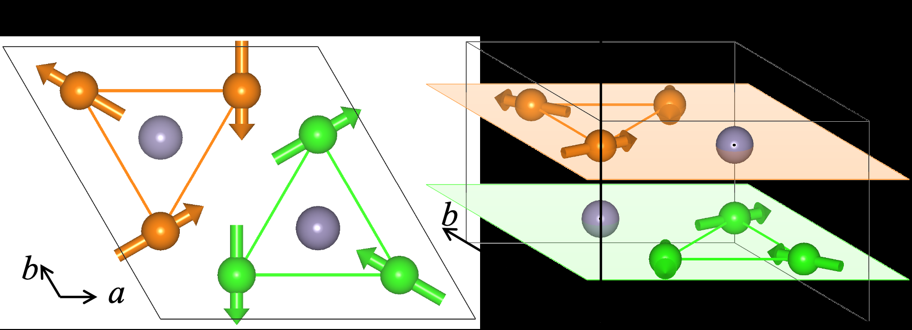
Figure 2: (a) Magnetic crystal structure of Mn 3 S n in coplanar configuration. (b) The modified POSCAR including magnetic moments. Figure 3: Screenshot of ‘ssg.out’. The SSG number and label are generated, and the redefined axes of spin space are also output explicitly.
B. Finding SSG operations and international symbol
The program IRSSG first determines the SSG magnetic configuration type (I: collinear; II: coplanar; III: noncopla- nar). Then, it finds the SSG operations of the subgroup G 0 . Intuitively, all SSG elements of G 0 must be contained in the direct product of the moment-part group A and the atomic-part group B ( i.e. , G 0 ≤ A × B ). The moment-part group A is an NPG determined solely by the magnetic moments. The atomic space group B is a CSG obtained by neglecting magnetic moments. All SSG operations are identified by find ssg operation.py using the spglib [ 49 ] and pymatgen [ 50 ] packages, and a dictionary variable ssg ops is generated. Additionally, a binary file ‘ssg.data’ is generated, which includes all operations of the full SSG G . This file is required for constructing character tables and computing band representations. Once ‘ssg.data’ is prepared with the operations of a CSG or an MSG (as a specific SSG case), IRSSG works for them as well. Then, based on all SSG operations, the SSG number and international symbol are determined by get ssg number.py and get ssg symbol.py, respectively. Since the spin space and lattice space are independent, the redefined spin- space coordinates ( x ′ , y ′ , z ′ ) are output, depending on the spin configuration provided as input. For type-I SSGs, the redefined z ′ axis is chosen to align with the spin direction. For type-II SSGs, the x ′ y ′ plane is defined by the spin plane. For type-III SSGs, the x ′ y ′ z ′ axes are redefined following the standard NPG convention on the HSP. Under Table III: Structure of the tuple variable cell obtained by the function read poscar is given below ( N is the total number of atoms). Index Type Description 0 numpy.ndarray[(3,3), float] lattice vectors ( t 1 , t 2 , t 3 ) of the magnetic crystal structure 1 numpy.ndarray[(N,3), float] fractional coordinates of atoms ( f 1 t 1 , f 2 t 2 , f 3 t 3 ) 2 list[int] species indices of atoms 3 list[str] element symbols of atoms 4 numpy.ndarray[(N,3), float] magnetic moments of atoms in Cartesian coordinates
8 the redefined coordinates, the spin space rotation becomes U α = ζ α ⊕ I 1 for type-I and U α = I 2 ⊕ ξ α for type-II. Here, I n is the n -dimensional identity, ξ α = ± 1, and ζ α is a 2 × 2 O (2) matrix. A screenshot of ‘ssg.out’ for Mn 3 S n with a coplanar configuration is shown in Fig. 3 .
C. Character tables at high-symmetry k points
We construct the character tables of the coirreps of the k -little groups LG ( k ) at all k points.
1. Obtaining the SSG k-little group
The SSG operations are read from ‘ssg.data’ by get ssg.f90. An SSG operation that leaves k invariant up to a reciprocal-lattice vector [Eq. (4)] belongs to the k -little group; this is implemented in kgroup.f90. All related variables are summarized in Table IV in detail.
2. Generating the character table of the k-little group
In this part, we use the Hamiltonian method to decompose the regular projective corep to obtain the projective coirreps, and finally obtain the linear coirreps, which are all done in file linear rep.f90. The related variable is listed in Table IV , while Ncoirrep and Ch table2 are valid only when aunt=2. The factor system ω is obtained from Eq. ( 7 ). The regular projective corep is then constructed as M i j ( O α ) = ω ( O α , O j ) δ O i , [ O α O j ] , O α is unitary , ω ( O α , O j ) δ O i , [ O α O j ] K , O α is anti-unitary , with O α , O i , O j , [ O α O j ] ∈ LG ( k ) (19) where K is the complex conjugation. The regular projective corep is completely reducible and decomposes as the direct sum of all inequivalent projective coirreps, M ∼ = ρ d ρ M ( ρ ) , where M ( ρ ) is the matrix of projective coirrep ρ , and d ρ is its multiplicity, equal to the dimension divided by the torsion of ρ . Thus, the projective coirreps are obtained by decomposing the regular projective corep using the Hamiltonian method. The results are written to ‘chart.dat’.
3. Obtaining compatibility relations
Due to subgroup relations between the SSG little groups of adjacent k points, the compatibility relations are generated accordingly. They are written to ‘chart.dat’ as well. Table IV: Brief summary of variables on SSG G and the little group LG ( k ). Variables Type Description SSG G num sym integer Total number of operations in SSG G ( i.e. , G/T 0 ) . Spin rot(3,3,num sym) real U α : spin part of operations O α ∈ G . Rot(3,3,num sym) integer R α : rotation part of operations O α ∈ G . Tau(3,num sym) real v α : translation part of operations O α ∈ G . LG ( k ) NumLG integer Total number of SSG operations in the little group LG ( k ). litt group(:) integer Indices of SSG operations belonging to LG ( k ). aunt integer Flag for (anti-)unitarity of LG ( k ), 1: unitary, 2: anti-unitary.
Nirrep Ch table1(Nirrep,NumLG/aunt) Ncoirrep Ch table2(Ncoirrep,NumLG/aunt)
complex integer complex
Description Total number of operations in SSG G ( i.e. , G/T 0 ) . U α : spin part of operations O α ∈ G . R α : rotation part of operations O α ∈ G . v α : translation part of operations O α ∈ G . Total number of SSG operations in the little group LG ( k ). Indices of SSG operations belonging to LG ( k ). Flag for (anti-)unitarity of LG ( k ), 1: unitary, 2: anti-unitary. Number of irreps of the unitary group of LG ( k ). Characters of the irreps for the unitary subgroup of LG ( k ). Total number of coirreps of LG ( k ). Characters of the unitary operations in the coirreps of LG ( k ).
9
1
0
7
-
1
0
8
1
0
6
1
0
5
1
0
6
(a) (b)
Figure 4: (a) Magnetic energy bands of Mn 3 S n with a type-II configuration. (b) Screenshot of ‘chart.dat’.
D. Computing the coirreps of magnetic energy bands
For each k point, we obtain the coirreps of all magnetic energy bands.
1. Computing the traces of the SSG operations in the k-little group
The coefficients C n k ζ j in Eq. ( 11 ) are stored in the WAVECAR generated by VASP and wfc.dat generated by QE. All coefficients are read by wave data.f90 and stored in the complex variables coeffa ( C n k ↑ j ) and coeffb ( C n k ↓ j ). To compute traces only, one can use the plane-wave wavefunctions directly. The characters of SSG elements of LG ( k ) are then computed using Eq. ( 13 ) for degenerate bands. In addition, IRSSG can compute the traces of SSG operations in the orthogonal localized Wannier basis via Eq. ( 17 ).
2. Assigning coirreps to magnetic energy bands
By comparing the obtained traces with the traces of the character tables, one can easily assign the coirreps, which is done in chrct.f90.
E. Outputting coirreps, character tables, and compatibility relations for the SSG system
The band characters and their coirreps are presented in the file ‘irssg.out’. Fig. 5 shows excerpts of this file for Mn 3 S n with a type-II configuration. This file first lists all operations of G/T 0 , each assigned an operation index. The character tables are output in the ‘chart.dat’ file along with compatibility relations. This file presents the character tables for irreps of the unitary subgroups of LG ( k ) at all k points with distinct labels, and provides the compatibility relations between adjacent k points. Fig. 4 (b) shows a screenshot of the ‘chart.dat’ file for Mn 3 S n with a type-II configuration.
IV. CAPABILITIES OF THE PROGRAM
Determining the representations of computed electronic bands is crucial for studying phenomena such as band crossings, high degeneracies, and k · p models and related effects. Tools such as Phonopy [ 51 , 52 ] and MOM2MSG [ 53 ] can identify the CSG or MSG of materials. For a magnetic structure, spinspg [ 54 ] and findspingroup [ 20 ] are available for identifying SSG operations and/or Chen-Liu symbol. However, tools for determining the (co)irreps of magnetic electronic states are lacking. Although the complete character tables for CSGs and MSGs are available in
10
(a)
(b)
(c)
Figure 5: The band coirreps determined by IRSSG, which are output in ‘irssg.out’. The first three columns give band indices, degeneracies, and energies (without subtracting the Fermi level E F ), respectively. Then the characters of unitary operations and coirrep labels are output. Panels (a)–(c) correspond to the two ∆ (DT) points (two dash-dotted lines in Fig. 4 (a)) and the K point. the literature [ 55 – 57 ], the character tables of SSGs are not yet broadly accessible. Our program IRSSG can obtain the k -little group and generate character tables for SSGs. It also determines the coirreps of magnetic energy bands based on DFT calculations or Wannier functions. Meanwhile, with a proper ‘ssg.data’, it also works for the 230 CSGs and 1651 MSGs. Thus, the corresponding ‘msg.data’ is automatically generated for studying the magnetic system in the presence of SOC. Furthermore, similar to POS2MSG [ 36 ], which can generate the magnetic structures with highest MSG symmetries, we developed an auxiliary tool, POS2SSG, to generate highest-SSG-symmetry magnetic configurations by assigning magnetic moments to magnetic atoms, thereby producing structures with SSG numbers specified by the user.
V. INSTALLATION AND USAGE OF IRSSG
IRSSG is an open-source package released on GitHub under the GNU General Public Licence 3.0, https://www.gnu.org/licenses/gpl-3.0.html. It can be downloaded directly from the public code archive: https://github.com/zjwang11/IRSSG. To build and install IRSSG, Python 3.8 or higher is required. The executable irssg and its dependencies are automatically downloaded and installed, and the coirreps of the m th– n th magnetic energy bands can be obtained by typing the following command:
$ pip install irssg $ irssg -ssg > ssg.out $ irssg -nb $m $n [ -tolE $dE ] > irssg.out
where -tolE sets the energy tolerance dE (0.001 eV by default) for identifying (near-)degenerate bands. Here, we take coplanar Mn 3 S n as an example to illustrate the procedure. The magnetic configuration [ 58 ] is shown in Fig. 2 (a). The corresponding modified POSCAR is shown in Fig. 2 (b). Then one can run the command ‘irssg -ssg > ssg.out’, which generates the ‘ssg.out’ (only the modified POSCAR is required as input), as shown in Fig. 3 . From this output, one can find that the SSG international symbol for the Mn 3 S n configuration is P 1 , 1 , 1 6 3 − 1 3 /m 1 m m c m (C I I 3 v ) with SSG number 194.1.6.1.P. In addition, the redefined coordinates in spin space, the spin part group P and the lattice part group H of the SSG are also presented. The elements ( {U ||R| v } ) of the SSG are generated. We first perform the self-consistent and band-structure DFT calculations for the magnetic configurations ( e.g. setting ‘NONCOLLINEAR=.TRUE.; LSORBIT=.FALSE.’ in INCAR for VASP). The wavefunctions must be output in the DFT calculation. The noncollinear band structure for Mn 3 S n is obtained in Fig. 4 (a). We can find that there might be two ‘crossing’ points around the Fermi level, which need to be confirmed by the SSG coirreps. Then one can use the command ‘irssg -nb 103 108 > irssg.out’ to obtain the SSG coirreps of 103-108 -th bands, with the results written to ‘irssg.out’. The character tables (including compatibility relations) for all k points are generated in ‘chart.dat’, whose screenshot is given in Fig. 4 (b). Explicitly, the screenshots of ‘irssg.out’ are given in Fig. 5 for the three k points (denoted by two brown dash-dot lines in Fig. 4 (a) and K), which indicate that the crossing at ZΓ is a 3-fold crossing point, formed by DT4 (106-th band) and DT6 (107-th and 108-th bands). The Dirac point at K forms a K6 coirrep, indicating that it is a symmetry-enforced, conventional twofold band-degeneracy point [ 18 ]. The coirrep matrices of the generators of LG (K) are D ( {E||M z | 0 , 0 , 1 2 } ) = −σ 0 , D ( {C − 1 3 z ||C 3 z | 0 , 0 , 0 } ) = 1 2 ( σ 0 − √ 3 iσ z ), D ( {C 2( √ 3 2 , 1 2 , 0) | |M y | 0 , 0 , 1 2 } ) = −iσ x , and D ( {M z ||P | 0 , 0 , 0 } ) = σ x K . Based on the coirrep matrices of the generators,
11
(a) GM8 GM8 GM8 GM7 D
T
1
D
T
1
D
T
2
D
T
2
(b) (c)
(d)
(e)
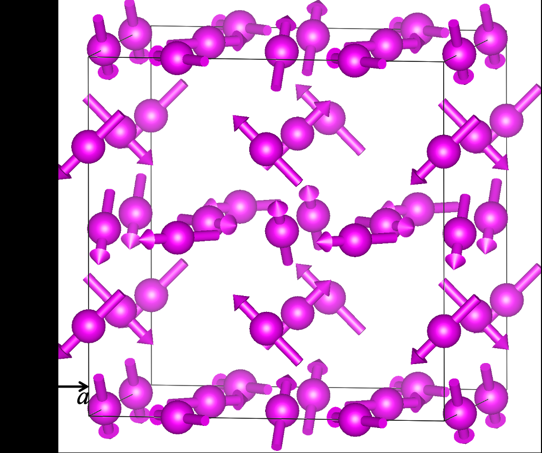
Figure 6: (a) Magnetic crystal structure of NpBi with a type-III configuration, where Np atoms are magnetic. (b) Magnetic energy bands of NpBi. (c) The fourfold nodal line of NpBi in the k z = 0 plane. SSG coirreps (d) and MSG coirreps (e) of the related two doubly degenerate bands. Being different from SSG coirreps, the ‘m’ is added as the prefix of MSG coirreps. the k · p effective model is also obtained for the SSG system via the invariant theory H ( k x , k y , k z ) = 0 b 1 k − + c 2 k 2 + b 1 k + + c 2 k 2 − 0 + [ a 1 + c 1 ( k 2 x + k 2 y ) + c 3 k 2 z ] σ 0 (20) where k ± = k x ± ik y , and the k · p parameters are a 1 = 9 . 0882eV, b 1 = 1 . 0768eV · ˚ A, c 1 = 1 . 9892eV · ˚ A 2 , c 2 = 1 . 3385eV · ˚ A 2 and c 3 = − 11 . 9826eV · ˚ A 2 . The parameters are directly obtained by using VASP2KP [ 59 ] in the DFT calculation. One can clearly see that it is a quasi-2D-Dirac point with linear dispersions in the xy plane, while it is quadratic (doubly degenerate) in the z direction. Only two Pauli matrices are allowed in the k · p Hamiltonian. A nontrivial π Berry phase of the circle surrounding it can be obtained by the 1D Wilson loop method.
VI. APPLICATIONS TO MAGNETIC MATERIALS
A. The fourfold nodal lines in NpBi
The noncoplanar magnetic configuration of NpBi [ 60 ] is illustrated in Fig. 6 (a). Its SSG international symbol F 2 , 2 , 2 m 1 ¯ 3 3 − 1 m m (T I II d ) and SSG number 225.4.6.2 are obtained by IRSSG. After the noncollinear DFT calculations in the absence of SOC, the band structure is obtained along MΓR (Fig. 6 (b)) and the wavefunctions ( e.g. WAVECAR in VASP) are written out as well, with the total number of electrons being 80. Using the command ‘irssg -nb 63 86 > irssg.out’, the coirreps are generated for 63-86 -th bands. We find that the crossing along MΓ is formed by DT1 and DT2. The crossing is fourfold degenerate. In addition, the fourfold crossing is part of the fourfold nodal line in the k z = 0 plane, as shown in Fig. 6 (c). Due to the presence of {C 3 (111) | |C 3 (111) | 0 , 0 , 0 } , the symmetry-related nodal lines appear in the k x = 0 and k y = 0 planes as well. The detailed coirrep analysis shows that the band inversion occurs between GM8- and GM7-coirrep bands at Γ, both of which are sixfold. The fourfold nodal lines are actually formed by this sixfold band inversion. All the generic bands are doubly degenerate due to the presence of two unitary SSG symmetries at an arbitrary k point, O α = {C 2 x | |E| 0 , 1 2 , 1 2 } and O β = {C 2 y ||E| 1 2 , 0 , 1 2 } , with the anti-commutation relation ( {Q α , Q β } = 0). Once SOC is included, the symmetry is reduced and must be described by a MSG, in which the spin part and the lattice part are closely coupled. Thus, only some of the SSG operations, whose spin part and lattice part contain the same proper rotation, are preserved in the MSG (including SOC). As a subgroup of the SSG, the ‘msg.data’ of MSG symmetry is automatically generated at the same time by the command ‘irssg -ssg’. One can obtain the MSG coirreps by the command ‘irssg -nb 79 82 -so > irmsg.out’ (reading ‘msg.data’ instead). This analysis is quite useful for the SOC-induced band splitting and other effects. The results show that the SSG coirrep DT1 becomes the MSG coreps mDT1+mDT2, and DT2 also becomes mDT1+mDT2, as shown in Fig. 6 (d)
12
(a) (b) (c)
DT5 SM3 DT2 DT 2 SM1 DT5 SM3
SM1 GM8 GM5
Figure 7: (a) Crystal structure of Eu 3 P bO. (b) Magnetic structure of Eu in Eu 3 P bO. (c) Magnetic energy bands of Eu 3 P bO. and (e). As a result, once SOC is included, the nodal line becomes fully gapped, since the crossing bands share the same MSG coreps.
B. The E F -enforced degenerate point in Eu 3 PbO
The crystal structure of Eu 3 P bO is shown in Fig. 7 (a), which is an anti-perovskite structure with Pb at the A site and O at the B site [ 61 ]. The noncoplanar magnetic configuration is illustrated in Fig. 7 (b), with SSG international symbol P m,m,m m 1 ¯ 3 3 m m (O I II h ) and SSG number 221.8.6.1 obtained by IRSSG. After the noncollinear calculations in the absence of SOC, the band structure and the wavefunctions are obtained along high-symmetry lines (as shown in Fig. 7 (c)). Using the command ‘irssg -nb 487 492 > irssg.out’, the coirreps are generated for bands 487- 492 ( N t ot = 488). We conclude that the crossing along ΓX is formed by DT2 (twofold) and DT5 (fourfold). The detailed analysis shows that the band inversion occurs between GM5 (fourfold) and GM8 (sixfold), resulting in a high-degeneracy point between N t ot and N t ot + 1 bands. The red line is the highest valence band, while the blue line is the lowest conduction band. All the bands are doubly degenerate due to the presence of two unitary SSG symmetries with the anti-commutation relation ( {C 2 x | |E| 1 2 , 1 2 , 0 } and {C 2 y ||E| 0 , 1 2 , 1 2 } ).
VII. CONCLUSIONS
In summary, we have developed an open-source software package – IRSSG – representing the first computational code to determine the coirreps of magnetic states in spin space groups. It first generates the SSG operations, numbers, and international symbols for magnetic crystal structures; second, it constructs character tables for high-symmetry k points; and finally, it computes the traces of SSG operations and assigns coirreps of the magnetic energy bands obtained from DFT codes. Detailed information is released on the HSP. In addition, it also works for the MSG symmetry once the SOC is included in the SSG systems. We further demonstrate how to use it to identify coirreps and high-degeneracy excitations in magnetic materials. This program does not restrict the user to a single DFT program or a single TB Hamiltonian. It works for the DFT codes, such as VASP and Quantum ESPRESSO, as well as any other code that has an interface to Wannier90. The program is very important for advancing research on the study of magnons, altermagnetism, magnetic topology, and novel high-degeneracy excitations in SSG systems.
Acknowledgment
Acknowledgment We thank Prof. Chen Fang and Dr. Yi Jiang for helpful discussions. This work was supported by the National Key R&D Program of China (Grant No. 2022YFA1403800), National Natural Science Foundation of China (Grant No. 12188101), and the Center for Materials Genome.
Appendix A: Comparison between different SSG notations
We provide a side-by-side comparison between our symbols output by IRSSG and Chen-Liu symbols of Ref. [20], as shown in Table S1. Chen-Liu symbols can be rather involved, as they are constructed within a classification scheme
13 that divides SSGs into three types: t -type, k -type, and g -type. We use the three materials discussed in the main text (Mn 3 S n, NpBi, and Eu 3 P bO), and additionally include CeAuAl 3 in Ref. [ 20 ]. Materials Chen-Liu symbol of Ref. [ 20 ] IRSSG symbol Mn 3 S n t -type: P 3 1 0 01 6 3 / 1 m 2 1 00 m 2 π / 3 c m 1 P 1 , 1 , 1 6 3 − 1 3 /m 1 m m c m (C I I 3 v ) NpBi g -type: F 1 m 3 1 1 11 ¯ 3 m 1 ¯ 10 m | (1 , 1 , 1; 2 0 01 , 2 0 10 , 2 1 00 ) F 2 , 2 , 2 m 1 ¯ 3 3 − 1 m m (T I II d ) Eu 3 P bO g -type: P 1 m 3 1 1 11 ¯ 3 m 0 1 ¯ 1 m | ( m 0 10 , m 0 01 , m 1 00 ) P m,m,m m 1 ¯ 3 3 m m (O I II h ) CeAuAl 3 k -type: P 1 4 1 m 1 m 4 1 0 01 1 2 1 2 1 4 m 1 I 4 − 1 4 − 1 4 4 1 m 1 m 1 (C I I 4 ) Table S1: Several magnetic materials, with their SSG symmetries represented in Chen-Liu symbol and in our symbol by IRSSG.
Appendix B: Derivation of the factor system arising from the translation part
Let O α = {U α | |R α | v α } , O β = {U β ||R β | v β } and O γ = {U α U β ||R α R β | ( R α v β + v α ) mod 1 } . We aim to verify that the translation-derived factor takes the form ω τ ( O α , O β ) = exp[ −i k · ( R α − det( U α ) ) v β ] , (B1) and to show how this factor arises from the relation between linear and projective representations. We relate the projective representation M and the linear representation D by a translational phase factor: D ( O α ) = exp( −i k · v α ) M ( O α ) . (B2) Using the usual multiplication law for the linear representations, D ( O α ) D ( O β ) = D ( {U α U β ||R α R β |R α v β + v α } ) , (B3) one expects the projective representations to satisfy a modified multiplication rule with a factor system, M ( O α ) M ( O β ) = ω τ ( O α , O β ) M ( O γ ) , (B4) We now derive ω τ by substituting Eq. ( B2 ) into the product M ( O α ) M ( O β ). When O α is unitary (so that det( U α ) = 1), a straightforward manipulation yields M ( O α ) M ( O β ) = exp[ i k · ( v α + v β )] D ( O α ) D ( O β ) = exp[ i k · ( v α + v β )] D ( O γ ) exp[ −i k · ( R α v β + v α − v γ )] = exp[ i k · ( v α + v β )] M ( O γ ) exp[ −i k · v γ ] exp[ −i k · ( R α v β + v α − v γ )] = exp[ i k · ( v β − R α v β )] M ( O γ ) (B5) from which the unitary case of Eq. ( B1 ) follows. When O α is anti-unitary (so that det( U α ) = − 1), one must account for the fact that both M ( O α ) and D ( O α ) reverse the sign of i , i.e. , M ( O α ) i = −i M ( O α ) and D ( O α ) i = −i D ( O α ) . Repeating the same substitution and keeping track of this sign change leads to M ( O α ) M ( O β ) = exp[ i k · ( v α − v β )] D ( O α ) D ( O β ) = exp[ i k · ( v α − v β )] exp[ −i k · ( R α v β + v α − v γ )] D ( O γ ) = exp[ i k · ( v α − v β )] exp[ −i k · ( R α v β + v α − v γ )] exp[ −i k · v γ ] M ( O γ ) = exp[ −i k · ( v β + R α v β )] M ( O γ ) (B6) This yields the anti-unitary case of Eq. ( B1 ). Combining Eqs. ( B5 ) and ( B6 ), we have thus shown that any linear representation D ( O α ) obeying Eq. ( B3 ) can be obtained from a projective representation M ( O α ) that satisfies Eq. ( B4 ) with the factor system given in Eq. ( B1 ). The two representations are related by the translational phase factor in Eq. ( B2 ).
14 Appendix C: ‘tbbox.in’ parameters
For tight-binding calculations, tbbox.in is required. A useful tool ‘gen tbbox.py’ is developed to generate tbbox.in from Wannier90 files directly, which is available at https://github.com/zjwang11/IRSSG . An example of Mn 3 S n with a type-II configuration is given below.
spinpol = False
spinpol = False # hr_name_up = sp . up_hr . dat # hr_name_dn = sp . dn_hr . dat hr_name = symm_hr . dat
proj :
proj : orbt = 2 spincov = 1 ntau = 8 0.838800 0.677599 0.161200 0.838800 0.838800 0.161200 0.161200 0.322401 0.322401 0.161200 0.677599 0.838800 0.333333 0.666667 0.666667 0.333333
end proj 0.250000 2.598077 1.5 0.750000 -2.598077 1.5 0.250000 -2.598077 1.5 0.750000 2.598077 1.5 0.250000 0.000000 -3.0 0.750000 0.000000 -3.0 0.250000 0.000000 0.0 0.750000 0.000000 0.0 0 0 0 0 0 0 0 0 1 1 1 1 1 1 2 2 5 5 5 5 5 5 3 3 ! x1 , x2 , x3 , m1 , m2 , m3 , itau , iorbit kpoint :
kpoint : kmesh = 10 Nk = 2
0 0 0 0.5 0 0 end kpoint unit_cell :
5.665000 -2.832500 0.000000 end unit_cell 0.000000 4.906034 0.000000 0.000000 0.000000 4.531000
1. spinpol: whether the magnetism of the system is collinear (type-I SSG) ( e.g. ‘ISPIN=2’ and ‘NON- COLLINEAR=.FALSE. in INCAR for VASP’). Default: False. 2. hr name: the name of the input file containing TB parameters, whose format should be the same as ‘wan- nier90 hr.dat’ generated by Wannier90. This parameter only works when spinpol=False. 3. hr name up: the name of the input file containing TB parameters with up spin. This parameter is valid for
spinpol=True.
4. hr name dn: the name of the input file containing TB parameters with down spin. This parameter is valid for
spinpol=True.
5. unit cell: 3 × 3 lattice matrix in Cartesian coordinates ( ˚ A). Each row is one direct lattice vector, in the order a , b , c . The 3-5 lines in POSCAR can be pasted here directly. 6. kpoint . . . end kpoint: defines a k-space path for band sampling. • kmesh: number of evenly spaced samples taken on each consecutive line segment between listed k-nodes. • Nk: number of k points that follow; the path is formed by connecting them in order. • k points list: k points given in fractional coordinates with respect to the reciprocal basis vectors b 1 , b 2 , b 3 . 7. proj: . . . end proj: defines the local-orbital projectors used to build the TB basis. Each projector line has
eight fields (x1, x2, x3, m1, m2, m3, itau, iorbit).
15 • orbt: convention for orbital ordering. It selects how each iorbit maps to concrete orbitals, as in Table S2 . • spincov: spinful basis ordering . 1 = orbit-major, spin-minor ( a ↑, b ↑, . . . , a ↓, b ↓, . . . ); 2 = spin-major, orbit-minor ( a ↑, a ↓, b ↑, b ↓, . . . ). • ntau: number of site lines that follow (i.e., the number of TB sites listed in this block). • Site lines: each line is (x1, x2, x3, m1, m2, m3, itau, iorbit) where x1, x2, x3 are fractional coor- dinates, m1, m2, m3 are magnetic moments in Cartesian coordinates, itau labels the atomic species/type, and iorbit selects the on-site orbital set according to orbt (see Table S2 ). Table S2: Local orbitals ordering in different conventions [ 29 ].
iorbit Convention 1 Convention 2
iorbit Convention 1 Convention 2 1 s s 3 p x , p y , p z p z , p x , p y 5 d x y , d y z , d x z , d x 2 − y 2 , d z 2 d z 2 , d x z , d y z , d x 2 − y 2 , d x y 4 s, p x , p y , p z s, p z , p x , p y 6 s, d x y , d y z , d x z , d x 2 − y 2 , d z 2 s, d z 2 , d x z , d y z , d x 2 − y 2 , d x y 8 p x , p y , p z , d x y , d y z , d x z , d x 2 − y 2 , d z 2 p z , p x , p y , d z 2 , d x z , d y z , d x 2 − y 2 , d x y 9 s, p x , p y , p z , d x y , d y z , d x z , d x 2 − y 2 , d z 2 s, p z , p x , p y , d z 2 , d x z , d y z , d x 2 − y 2 , d x y 7 f x yz , f 5 x 3 − xr 2 , f 5 y 3 − yr 2 , f 5 z 3 − zr 2 , f x ( y 2 − z 2 ) , f y ( z 2 − x 2 ) , f z ( x 2 − y 2 ) f z 3 , f x z 2 , f y z 2 , f z ( x 2 − y 2 ) , f x yz , f x ( x 2 − 3 y 2 ) , f y (3 x 2 − y 2 ) [1] N. A. Benedek and C. J. Fennie, Phys. Rev. Lett. 106 , 107204 (2011), URL https://link.aps.org/doi/10.1103/ PhysRevLett.106.107204 .
PhysRevLett.106.107204. [2] S. Zhang, Y. Liu, Z. Sun, X. Chen, B. Li, S. L. Moore, S. Liu, Z. Wang, S. E. Rossi, R. Jing, et al., Nature Communications 14 , 6200 (2023), ISSN 2041-1723, URL https://doi.org/10.1038/s41467-023-41773-x. [3] G. Yu, J. Ji, Y. Chen, C. Xu, and H. J. Xiang, Phys. Rev. Lett. 134 , 016801 (2025), URL https://link.aps.org/doi/ 10.1103/PhysRevLett.134.016801.
10.1103/PhysRevLett.134.016801 . [4] E. Galiffi, G. Carini, X. Ni, G. ´ Alvarez P´erez, S. Yves, E. M. Renzi, R. Nolen, S. Wasserroth, M. Wolf, P. Alonso-Gonzalez, et al., Nature Reviews Materials 9 , 9 (2024), ISSN 2058-8437, URL https://doi.org/10.1038/s41578-023-00620-7 . [5] L. Shu, Y. Xia, B. Li, L. Peng, H. Shao, Z. Wang, Y. Cen, H. Zhu, and H. Zhang, npj Computational Materials 10 , 2 (2024), ISSN 2057-3960, URL https://doi.org/10.1038/s41524-023-01162-w . [6] Y.-Q. Lin, S.-H. Cao, C.-E. Hu, H.-Y. Geng, and X.-R. Chen, Phys. Rev. B 110 , 075414 (2024), URL https://link.aps. org/doi/10.1103/PhysRevB.110.075414 .
org/doi/10.1103/PhysRevB.110.075414. [7] H. Zhang, C.-X. Liu, X.-L. Qi, X. Dai, Z. Fang, and S.-C. Zhang, Nature Physics 5 , 438 (2009), ISSN 1745-2481, publisher: Nature Publishing Group, URL https://www.nature.com/articles/nphys1270. [8] T. H. Hsieh, H. Lin, J. Liu, W. Duan, A. Bansil, and L. Fu, Nature Communications 3 , 982 (2012), ISSN 2041-1723, URL https://doi.org/10.1038/ncomms1969.
https://doi.org/10.1038/ncomms1969. [9] L. Elcoro, B. J. Wieder, Z. Song, Y. Xu, B. Bradlyn, and B. A. Bernevig, Nature Communications 12 , 5965 (2021), ISSN 2041-1723, URL https://doi.org/10.1038/s41467-021-26241-8. [10] J. Yao, R. Zhang, S. Zhang, H. Sheng, Y. Shi, Z. Fang, H. Weng, and Z. Wang, Phys. Rev. B 111 , L041117 (2025), URL
https://link.aps.org/doi/10.1103/PhysRevB.111.L041117 .
https://link.aps.org/doi/10.1103/PhysRevB.111.L041117. [11] S. Ono, Y. Yanase, and H. Watanabe, Phys. Rev. Res. 1 , 013012 (2019), URL https://link.aps.org/doi/10.1103/
[11] S. Ono, Y. Yanase, and H. Watanabe, Phys. Rev. Res. 1 , 013012 (2019), URL https://link.aps.org/doi/10.1103/ PhysRevResearch.1.013012. [12] S. Ono and K. Shiozaki, Phys. Rev. X 12 , 011021 (2022), URL https://link.aps.org/doi/10.1103/PhysRevX.12.011021. [13] S. Ono, H. C. Po, and H. Watanabe, Science Advances 6 , eaaz8367 (2020), URL https://www.science.org/doi/abs/10. 1126/sciadv.aaz8367.
1126/sciadv.aaz8367. [14] C. J. Bradley and B. L. Davies, Rev. Mod. Phys. 40 , 359 (1968), URL https://link.aps.org/doi/10.1103/RevModPhys.
40.359.
40.359. [15] W. F. Brinkman and R. J. Elliott, Proceedings of the Royal Society of London. Series A. Mathematical and Physical
Sciences 294, 343 (1966), URL https://royalsocietypublishing.org/doi/abs/10.1098/rspa.1966.0211 .
Sciences 294 , 343 (1966), URL https://royalsocietypublishing.org/doi/abs/10.1098/rspa.1966.0211. [16] D. Litvin and W. Opechowski, Physica 76 , 538 (1974), ISSN 0031-8914, URL https://www.sciencedirect.com/science/
article/pii/0031891474901578.
article/pii/0031891474901578. [17] D. B. Litvin, Foundations of Crystallography 33 , 279 (1977). [18] P. Liu, J. Li, J. Han, X. Wan, and Q. Liu, Phys. Rev. X 12 , 021016 (2022), URL https://link.aps.org/doi/10.1103/
PhysRevX.12.021016.
PhysRevX.12.021016. [19] Z. Xiao, J. Zhao, Y. Li, R. Shindou, and Z.-D. Song, Phys. Rev. X 14 , 031037 (2024), URL https://link.aps.org/doi/
10.1103/PhysRevX.14.031037.
16 [20] X. Chen, J. Ren, Y. Zhu, Y. Yu, A. Zhang, P. Liu, J. Li, Y. Liu, C. Li, and Q. Liu, Phys. Rev. X 14 , 031038 (2024), URL
https://link.aps.org/doi/10.1103/PhysRevX.14.031038 .
https://link.aps.org/doi/10.1103/PhysRevX.14.031038. [21] Y. Jiang, Z. Song, T. Zhu, Z. Fang, H. Weng, Z.-X. Liu, J. Yang, and C. Fang, Phys. Rev. X 14 , 031039 (2024), URL
https://link.aps.org/doi/10.1103/PhysRevX.14.031039 .
https://link.aps.org/doi/10.1103/PhysRevX.14.031039. [22] A. Corticelli, R. Moessner, and P. A. McClarty, Phys. Rev. B 105 , 064430 (2022), URL https://link.aps.org/doi/10.
1103/PhysRevB.105.064430.
1103/PhysRevB.105.064430. [23] X. Chen, Y. Liu, P. Liu, Y. Yu, J. Ren, J. Li, A. Zhang, and Q. Liu, Nature 640 , 349 (2025), ISSN 1476-4687, URL
https://doi.org/10.1038/s41586-025-08715-7 .
https://doi.org/10.1038/s41586-025-08715-7. [24] X. Feng and Z. Zhang, Phys. Rev. B 111 , 054520 (2025), URL https://link.aps.org/doi/10.1103/PhysRevB.111.
054520 . [25] L. ˇ Smejkal, J. Sinova, and T. Jungwirth, Phys. Rev. X 12 , 031042 (2022), URL https://link.aps.org/doi/10.1103/
PhysRevX.12.031042.
PhysRevX.12.031042 . [26] L. ˇ Smejkal, J. Sinova, and T. Jungwirth, Phys. Rev. X 12 , 040501 (2022), URL https://link.aps.org/doi/10.1103/
PhysRevX.12.040501.
PhysRevX.12.040501. [27] Z. Liu, M. Wei, W. Peng, D. Hou, Y. Gao, and Q. Niu, Phys. Rev. X 15 , 031006 (2025), URL https://link.aps.org/
doi/10.1103/PhysRevX.15.031006.
doi/10.1103/PhysRevX.15.031006. [28] Y. Liu, X. Chen, Y. Yu, J. Etxebarria, J. M. Perez-Mato, and Q. Liu, Symmetry classification of magnetic orders using
oriented spin space groups (2026), 2506.20739, URL https://arxiv.org/abs/2506.20739 .
oriented spin space groups (2026), 2506.20739, URL https://arxiv.org/abs/2506.20739. [29] J. Gao, Q. Wu, C. Persson, and Z. Wang, Comput. Phys. Commun. 261 , 107760 (2021), ISSN 0010-4655, code available at https://github.com/zjwang11/IRVSP. [30] G. Kresse and J. Furthmu¨ller, Phys. Rev. B 54 , 11169 (1996), URL https://link.aps.org/doi/10.1103/PhysRevB.54. 11169.
11169. [31] G. Kresse and J. Furthmu¨ller, Computational Materials Science 6 , 15 (1996), ISSN 0927-0256, URL https://www.
sciencedirect.com/science/article/pii/0927025696000080.
sciencedirect.com/science/article/pii/0927025696000080. [32] P. Giannozzi, S. Baroni, N. Bonini, M. Calandra, R. Car, C. Cavazzoni, D. Ceresoli, G. L. Chiarotti, M. Cococcioni, I. Dabo, et al., Journal of Physics: Condensed Matter 21 , 395502 (2009), URL https://doi.org/10.1088/0953-8984/ 21/39/395502.
21/39/395502. [33] P. Giannozzi, O. Andreussi, T. Brumme, O. Bunau, M. Buongiorno Nardelli, M. Calandra, R. Car, C. Cavazzoni, D. Ceresoli, M. Cococcioni, et al., Journal of Physics: Condensed Matter 29 , 465901 (2017), URL https://doi.org/
10.1088/1361-648X/aa8f79.
10.1088/1361-648X/aa8f79. [34] N. Marzari, A. A. Mostofi, J. R. Yates, I. Souza, and D. Vanderbilt, Rev. Mod. Phys. 84 , 1419 (2012), URL https:
//link.aps.org/doi/10.1103/RevModPhys.84.1419.
//link.aps.org/doi/10.1103/RevModPhys.84.1419. [35] A. A. Mostofi, J. R. Yates, G. Pizzi, Y.-S. Lee, I. Souza, D. Vanderbilt, and N. Marzari, Computer Physics Communications
185, 2309 (2014), ISSN 0010-4655, URL https://www.sciencedirect.com/science/article/pii/S001046551400157X .
185 , 2309 (2014), ISSN 0010-4655, URL https://www.sciencedirect.com/science/article/pii/S001046551400157X. [36] J. Gao, Z. Guo, H. Weng, and Z. Wang, Phys. Rev. B 106 , 035150 (2022), website at https://tm.iphy.ac.cn/TopMat_ 1651msg.html, URL https://link.aps.org/doi/10.1103/PhysRevB.106.035150. [37] M. G. Vergniory, L. Elcoro, C. Felser, N. Regnault, B. A. Bernevig, and Z. Wang, Nature 566 , 480 (2019), ISSN 1476-4687, URL https://doi.org/10.1038/s41586-019-0954-4. [38] J. Gao, Y. Qian, H. Jia, Z. Guo, Z. Fang, M. Liu, H. Weng, and Z. Wang, Science Bulletin 67 , 598 (2022), ISSN 2095-
9273, website at https://tm.iphy.ac.cn/UnconvMat.html , URL https://www.sciencedirect.com/science/article/ pii/S2095927321008045.
pii/S2095927321008045. [39] Z. Song, A. Z. Yang, Y. Jiang, Z. Fang, J. Yang, C. Fang, H. Weng, and Z.-X. Liu, Phys. Rev. B 111 , 134407 (2025), URL
https://link.aps.org/doi/10.1103/PhysRevB.111.134407 .
https://link.aps.org/doi/10.1103/PhysRevB.111.134407. [40] Z.-Y. Yang, J. Yang, C. Fang, and Z.-X. Liu, Journal of Physics A: Mathematical and Theoretical 54 , 265202 (2021), URL
https://doi.org/10.1088/1751-8121/abfffc .
https://doi.org/10.1088/1751-8121/abfffc. [41] S. K. Kim, Journal of Mathematical Physics 25 , 2125 (1984), ISSN 0022-2488, URL https://doi.org/10.1063/1.526419. [42] P. Blaha, K. Schwarz, F. Tran, R. Laskowski, G. K. H. Madsen, and L. D. Marks, The Journal of Chemical Physics 152 , 074101 (2020), ISSN 0021-9606, URL https://doi.org/10.1063/1.5143061. [43] K. Schwarz, P. Blaha, and G. Madsen, Computer Physics Communications 147 , 71 (2002), ISSN 0010-4655, proceedings of the Europhysics Conference on Computational Physics Computational Modeling and Simulation of Complex Systems, URL https://www.sciencedirect.com/science/article/pii/S0010465502002060. [44] T. Ozaki and H. Kino, Phys. Rev. B 72 , 045121 (2005), URL https://link.aps.org/doi/10.1103/PhysRevB.72.045121. [45] T. Ozaki and H. Kino, Phys. Rev. B 69 , 195113 (2004), URL https://link.aps.org/doi/10.1103/PhysRevB.69.195113. [46] T. Ozaki, Phys. Rev. B 67 , 155108 (2003), URL https://link.aps.org/doi/10.1103/PhysRevB.67.155108. [47] J. C. Slater and G. F. Koster, Phys. Rev. 94 , 1498 (1954), URL https://link.aps.org/doi/10.1103/PhysRev.94.1498. [48] M. Willatzen and L. C. L. Y. Voon, The kp method: electronic properties of semiconductors , vol. 1 (Springer, 2009). [49] A. Togo, K. Shinohara, and I. Tanaka, Science and Technology of Advanced Materials: Methods 4 , 2384822 (2024), URL
https://doi.org/10.1080/27660400.2024.2384822 .
https://doi.org/10.1080/27660400.2024.2384822. [50] S. P. Ong, W. D. Richards, A. Jain, G. Hautier, M. Kocher, S. Cholia, D. Gunter, V. L. Chevrier, K. A. Persson, and G. Ceder, Computational Materials Science 68 , 314 (2013), ISSN 0927-0256, URL https://www.sciencedirect.com/
G. Ceder, Computational Materials Science 68 , 314 (2013), ISSN 0927-0256, URL https://www.scie science/article/pii/S0927025612006295. [51] A. Togo, L. Chaput, T. Tadano, and I. Tanaka, J. Phys. Condens. Matter 35 , 353001 (2023). [52] A. Togo, J. Phys. Soc. Jpn. 92 , 012001 (2023). [53] R. Zhang, Z. Sheng, and Z. Wang, Mom2ssg , code available at https://github.com/zjwang11/TopMat.
17 [54] K. Shinohara, A. Togo, H. Watanabe, T. Nomoto, I. Tanaka, and R. Arita, Acta Cryst. A 80 , 94 (2024), URL https: //doi.org/10.1107/S2053273323009257.
//doi.org/10.1107/S2053273323009257. [55] M. I. Aroyo, J. M. Perez-Mato, C. Capillas, E. Kroumova, S. Ivantchev, G. Madariaga, A. Kirov, and H. Wondratschek, Zeitschrift fu¨r Kristallographie - Crystalline Materials 221 , 15 (2006), URL https://doi.org/10.1524/zkri.2006.221.
Zeitschrift fu¨r Kristallographie - Crystalline Materials 221 , 15 (2006), URL https://doi.org/10.1524/zkri.2006.221. 1.15. [56] M. I. Aroyo, A. Kirov, C. Capillas, J. M. Perez-Mato, and H. Wondratschek, Acta Crystallographica Section A 62 , 115 (2006), URL https://doi.org/10.1107/S0108767305040286. [57] M. I. Aroyo, J. M. Perez-Mato, D. Orobengoa, E. Tasci, G. de la Flor, and A. Kirov, Bulg. Chem. Commun 43 , 183 (2011). [58] P. J. Brown, V. Nunez, F. Tasset, J. B. Forsyth, and P. Radhakrishna, Journal of Physics: Condensed Matter 2 , 9409 (1990), URL https://doi.org/10.1088/0953-8984/2/47/015. [59] S. Zhang, H. Sheng, Z.-D. Song, C. Liang, Y. Jiang, S. Sun, Q. Wu, H. Weng, Z. Fang, X. Dai, et al., Chin. Phys. Lett. 40 ,
127101 (2023), website at https://www.vasp2kp.com/ , URL https://dx.doi.org/10.1088/0256-307X/40/12/127101 .
127101 (2023), website at https://www.vasp2kp.com/, URL https://dx.doi.org/10.1088/0256-307X/40/12/127101. [60] P. Burlet, F. Bourdarot, J. Rossat-Mignod, J. Sanchez, J. Spirlet, J. Rebizant, and O. Vogt, Physica B: Condensed Matter
180-181, 131 (1992), ISSN 0921-4526, URL https://www.sciencedirect.com/science/article/pii/092145269290683J .
180-181 , 131 (1992), ISSN 0921-4526, URL https://www.sciencedirect.com/science/article/pii/092145269290683J. [61] M. M. Hirschmann, A. S. Gibbs, F. Orlandi, D. Khalyavin, P. Manuel, V. Abdolazimi, A. Yaresko, J. Nuss, H. Takagi, A. P. Schnyder, et al., Phys. Rev. Mater. 6 , 114202 (2022), URL https://link.aps.org/doi/10.1103/PhysRevMaterials.6.