⬇ Download Markdown · ⬇ Download LaTeX · ⬇ original · view original · CSV: table 1, table 2, table 3, table 4, table 5, table 6, table 7, table 8, table 9, table 10, table 11, table 12, table 13, table 14, table 15, table 16, table 17
High-Throughput Quantification of Altermagnetic Band Splitting
Ali Sufyan, 1, 2, 3 Brahim Marfoua, 4 J. Andreas Larsson, 3, 5 Erik van Loon, 1, 2 and Rickard Armiento 4
1 NanoLund and Division of Mathematical Physics, Department of Physics, Lund University, SE-221 00 Lund, Sweden
2 Wallenberg Initiative Materials Science for Sustainability, Department of Physics, Lund University, SE-221 00 Lund, Sweden 3 Applied Physics, Division of Materials Science, Department of Engineering Sciences and Mathematics,
Luleå University of Technology, SE-971 87 Luleå Sweden
4 Department of Physics, Chemistry and Biology, Linköping University, SE-581 83 Linköping, Sweden 5 Wallenberg Initiative Materials Science for Sustainability, Luleå University of Technology, SE-971 87 Luleå Sweden
Altermagnetism represents a recently established class of collinear magnetism that combines zero net magnetization with momentum-dependent spin polarization, enabled by symmetry constraints rather than spin-orbit coupling. This distinctive behavior gives rise to sizable spin splitting even in materials composed of light, earth-abundant elements, offering promising prospects for nextgeneration spintronics applications. Here, we present a comprehensive high-throughput screening of the 2287 entiries comprising the MAGNDATA database, integrating symmetry analysis with spinpolarized density functional theory (DFT) calculations to identify and characterize altermagnetic candidates. Our workflow investigates the collinear structures in the data set and collinear versions of the ones reported to be non-collinear, uncovering 180 materials exhibiting significant spin splitting, spanning both metallic and semiconducting systems. Detailed results are available for all 180 materials, but we also particularly discuss UCr 2 Si 2 C, NbMnP, and YRuO 3 as representative cases with large spin splitting. Furthermore, comparison with the Computational 2D Materials Database (C2DB) and the AiiDA 2D repository gives 9 bulk altermagnets with chemically equivalent 2D counterparts linked to the same ICSD parent entry. Crucially, our momentum-resolved analysis reveals that the spin splitting varies strongly across the Brillouin zone, and that the maximal splitting tends to occur away from the high-symmetry paths, a result that directly informs and guides future photoemission experiments. By expanding the catalog of known altermagnets, this work lays a robust foundation for future experimental and theoretical advances in spintronics and quantum materials discovery.
Altermagnetism has recently emerged as a distinct magnetic phase that expands beyond the traditional classifications of ferromagnetism (FM) and antiferromagnetism (AFM) [1–3]. The concept was initially introduced through theoretical predictions in rutile AFM RuO 2 in 2019 [4], and subsequently gained significant attention through systematic investigations of its distinctive characteristics in 2022, at which point the term “altermagnetism” was formally established [1, 2]. Conventional FM materials exhibit a net magnetization due to parallel alignment of spins, breaking time-reversal symmetry (TRS) uniformly throughout the crystal. In contrast, traditional AFMs have globally compensated spin arrangements with adjacent spins oriented antiparallel, thereby generating no net magnetization and typically enforcing spin degeneracy in their electronic band structure due to symmetry operations combining inversion or translational symmetry with TRS.
Altermagnets, however, possess globally compensated magnetization similar to AFMs but uniquely exhibit momentum-dependent spin polarization reminiscent of FM materials [1–12]. The essential distinction arises from the symmetry relations between their spin sublattices: in altermagnets, opposite-spin sublattices are related by rotation symmetries combined with TRS, rather than translation or inversion symmetries. This crucial difference in symmetry leads to nonrelativistic spin splitting of electronic bands, breaking Kramers degeneracy without the necessity of spin-orbit coupling (SOC) [4, 6, 7, 10, 13, 14]. In conventional AFMs, symmetry-enforced degeneracies typically prevent such splitting, while altermagnetic symmetry permits momentum-dependent spin-split bands that retain overall global spin compensation. Critically, because this spin splitting does not require SOC, altermagnetic behavior can manifest significantly even in materials composed of lighter, more earth-abundant elements like Fe and Mn. This broadens the scope for material discovery and significantly reduces reliance on heavier, expensive, or rare elements typically needed for SOC-driven phenomena [15]. Experimentally confirmed altermagnets now encompass diverse systems, from insulating compounds like CuF 2 [1], MnF 2 [7], and MnTe [14] to metallic materials such as RuO 2 [16], Mn 5 Si 3 [17], and CrSb [18]. These materials have demonstrated compelling and technologically relevant phenomena, including anomalous Hall effects (AHE), spin-polarized conductivity, spin-transfer torque, tunneling magnetoresistance, and giant magnetoresistance, which are essential ingredients for future spintronic applications [2, 19–24]. Consequently, the identification and characterization of alter2 magnetic materials represent a transformative advancement in magnetism and spintronics, sparking intensive research efforts aimed at uncovering new materials, elucidating underlying physical principles, and developing practical applications for this emerging class of magnetic materials.
However, discovering new altermagnets with significant spin splitting through trial-and-error experimental approaches is inherently challenging and resource-intensive. To overcome this limitation, highthroughput computational screening, leveraging reliable first-principles density functional theory (DFT) calculations, has emerged as an efficient and powerful methodology. This approach enables the rapid and systematic exploration of large material databases for candidates exhibiting desirable characteristics. Some recent efforts have used the MAGNDATA database [25, 26] for this purpose (see Sec. V for a comparison) with a focus on specific subclasses, such as metallic altermagnets or magnonic excitations in collinear systems, or using other selection criteria [27–29]. In this present work, we undertake an exhaustive and systematic high-throughput screening of the entire MAGNDATA database, including collinear versions of the non-collinear entries, without constraints to specific classes or properties, aiming to identify and comprehensively characterize all potential altermagnetic candidates. Through this extensive computational investigation, we successfully discover numerous previously unreported altermagnetic materials, validate several known candidates, and provide robust theoretical frameworks for future experimental realizations. This comprehensive approach not only significantly enhances the current understanding of altermagnetic phenomena but also expands the available pool of materials for next-generation spintronic devices, highlighting the critical importance and novelty of this study.
We present a rigorous two-stage high-throughput computational screening workflow for the systematic identification of candidate altermagnetic materials, summarized schematically in Fig. 1. In the first stage of screening (Fig. 1a), we retrieved the March 11, 2025 state of the MAGNDATA database hosted by the Bilbao Crystallographic Server [25, 26, 30]. This database contains 2287 published magnetic structures with crystal structures and magnetic configurations primarily obtained via experimental characterization.
These magnetic materials were subsequently analyzed using the recently developed computational tool amcheck [31]. Amcheck operationalizes the symmetry-based theoretical framework underpinning altermagnetism by assessing symmetry operations relating spin-up and spin-down magnetic sublattices. Specifically, the algorithm evaluates whether the magnetic sublattices can be mapped onto each other through a spatial inversion or lattice translation combined with a spin-flip operation. If such mappings are universally applicable to all magnetic atoms, the material is pure AFM since these symmetry operations guarantee spin degeneracy across the electronic band structure. Conversely, the absence of such inversion or translation symmetries, coupled with the presence of alternative symmetry operations (e.g., rotational or mirror symmetries), indicates altermagnetism. This condition implies the presence of symmetry-protected spin splitting in the band structure despite zero net magnetization. The advantage of amcheck lies in its reliance solely on crystallographic and magnetic structural information, circumventing the need for computationally intensive electronic structure calculations. Consequently, it serves as a rapid, efficient, and theoretically robust tool ideally suited to large-scale, high-throughput screenings. The symmetry analysis, both internally in amcheck and for the details we report in the supplementary materials uses Spglib [32, 33].
We used Pymatgen [34] to read the mcif files from MAGNDATA. We applied amcheck to all the collinear structures, which resulted in 157 candidate altermagnetic materials. We then applied amcheck to collinear versions of all noncollinear materials, where we aligned the spins by the algorithm used by Pymatgen when converting a magnetic moment to a scalar: the magnitude of the magnetic moment is retained and the sign assigned by projecting the moment onto a standard axis. The standard axis is arbitrarily chosen to always have the direction defined by the Cartesian vec-
collinear variants are introduced solely to enable a uniform high-throughput screening; we do not assess their energetic stability relative to the noncollinear ground state. This resulted in 131 additional candidates. Overall, we obtained a total of 288 potential AM materials from the MAGNDATA database (157 collinear and 131 noncollinear). Eliminating duplicated structures based on chemical composition and space group, the final set was 188 candidates suitable for further computational examination.
In the second screening phase (Fig. 1b), input files for spin-polarized self-consistent field (SCF) and nonself-consistent field (non-SCF) DFT calculations were systematically generated using Pymatgen and the Highthroughput toolkit (httk ) [35]. The workflow manager in httk provides a powerful, flexible automation framework specifically tailored for large-scale computational workflows, significantly enhancing computational efficiency. Importantly, magnetic orders and initial magnetic moments of atoms were directly extracted from MAGNDATA’s mcif files, ensuring consistency with experimentally established configurations. In cases where the reported local magnetic moments were particularly small (e.g., below 1 µ B /atom), we initialized the corresponding magnetic moments to a slightly higher value (typically 1 µ B ) to avoid artificial quenching during SCF relaxation.
The resulting spin-polarized SCF calculations, per3
MAGNDATA
.mcifs 2287 Magnetic
Materials
Fail amcheck
288 materials
Filter duplication Fail 198 candidate altermagnets 198 candidate altermagnets DFT input files Pymatgen Httk
Spin-polarized
DFT SCF VASP
NSCF DFT kmesh x2 VASP Δ>26 meV |E-E F |<3 eV Metals 22 Semiconductors 158 Altermagnetic
database Band structure
on hs-path 180 confirmed altermagnets VASP FIG. 1. Two-stage high-throughput computational workflow to identify candidate altermagnetic materials (AMs). (a) Initial screening selects experimentally characterized magnetic materials from the MAGNDATA database. Symmetry analysis via amcheck followed by deduplication filtering step, yielding a final set of 198 unique AM candidates. (b) In-depth computational verification using spin-polarized DFT calculations (VASP, pymatgen, and httk ). Materials exhibiting spin splitting (≥ 26 meV within ±3 eV of E F ) are confirmed as AM and included in the final database.
formed using the Vienna Ab-initio Simulation Package (VASP) [36–38], were analyzed to identify meaningful spin-splitting. To select only robust altermagnets, a minimum spin-splitting magnitude of 26 meV was used as a selection criterion and this splitting has to occur within an energy window of ±3 eV around the Fermi level. Figure S1 shows the distribution of ∆ max across the screened set and supports adopting 26 meV as a physically motivated lower bound, comparable to the room-temperature thermal energy scale (k B T ≈ 26 meV).
Based on these criteria, 180 materials were validated as exhibiting significant spin-splitting and advanced to the final characterization step, while the remaining candidates were discarded. Detailed electronic band structure calculations were subsequently conducted for these selected 180 altermagnets, enabling direct visualization and confirmation of spin-up and spin-down band splittings. Because magnetic symmetry can enforce nodal manifolds where the nonrelativistic splitting vanishes on many high-symmetry lines/planes, we evaluate ∆(k) on dense Brillouin-zone meshes (and fixed-k z slices when needed), rather than relying solely on conventional highsymmetry paths, to reliably capture ∆ max . In these computations, the magnetic moments were assumed to be in a collinear configuration, a commonly adopted simplification in high-throughput studies, which is sufficient for identifying the essential altermagnetic characteristics.
To further quantify the spin splitting, we computed both the average and volumetric spin-splitting metrics. The average spin splitting ⟨∆⟩ is defined as the mean of the maximum spin splitting across all k-points with eigenstates lying within a ±3 eV window around the Fermi level,
where W k is the set of bands at k within the energy window, and N is the number of contributing k-points.
The volumetric spin-splitting fraction F ∆ captures the fraction of bands and the portion of the Brillouin zone exhibiting appreciable spin splitting:
where w k is the k-point weight, M k is the number of bands within the energy window at k, and Θ is the Heaviside function applied with a small cutoff (e.g., 10 meV) to suppress numerical noise.
Note that the calculations are performed using the usual scalar-relativistic projector augmented-wave (PAW) pseudopotentials distributed with VASP, but we do not otherwise include spin–orbit coupling (SOC) or other relativistic corrections. This defines the nonrelativistic baseline for spin splitting in altermagnets, where the essential effect arises from exchange and crystalline symmetry rather than relativistic interactions. For compounds containing heavy 5d or 5f elements, however, SOC can strongly influence electronic phases [39] and consequently affect the magnitude of the spin splitting. The explicit inclusion of SOC in high-throughput workflows is computationally demanding and, in heavyelement systems, may also lead to convergence difficulties. Hence, in particular our results for heavy-element 4 compounds, which are expected to be more sensitive to these effects, may need further investigation for the contribution from SOC.
Summarized in Table II are the key properties of the top candidate materials identified through our highthroughput screening, including their maximum, average, and volumetric spin-splitting magnitudes (∆F ), electronic band gaps, Hubbard U parameters, and minimum elemental abundances. Among these, six altermagnets, CrSb, MnTe, CrSe, RuO 2 , Ca(Al 2 Fe) 4 , and UCr 2 Si 2 C, exhibit particularly pronounced spin-band splitting. Notably, experimental evidence for altermagnetism in CrSb [18], MnTe [40], and RuO 2 [16] has recently been presented, providing strong validation for the predictive capability of our computational framework. In the following sections, we focus on three representative cases: the metallic altermagnets UCr 2 Si 2 C and MnNbP, and the semiconducting altermagnet YRuO 3 , each exhibiting spin-splitting features and serving as compelling examples of the diverse electronic characteristics accessible within the altermagnetic landscape.
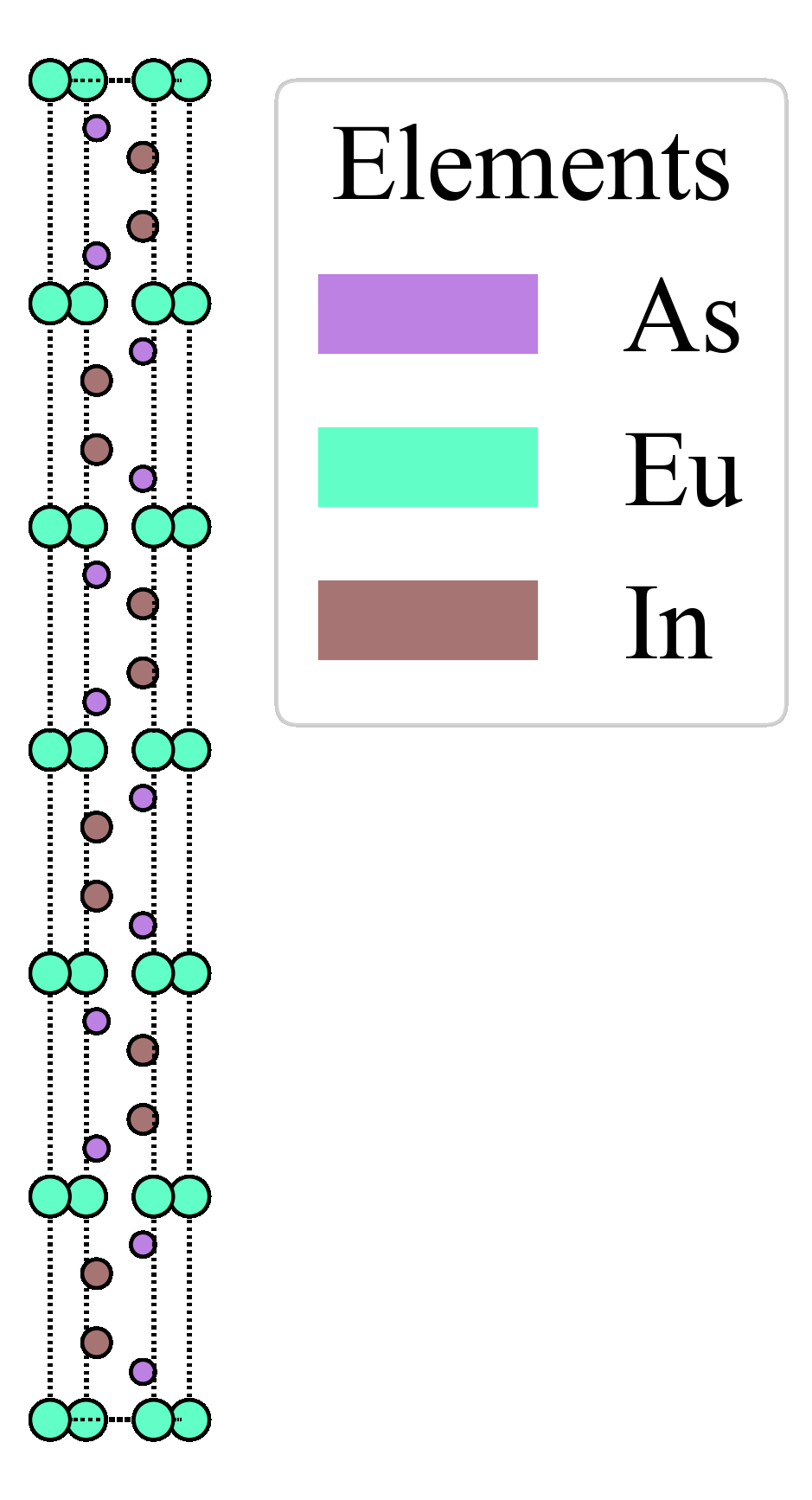
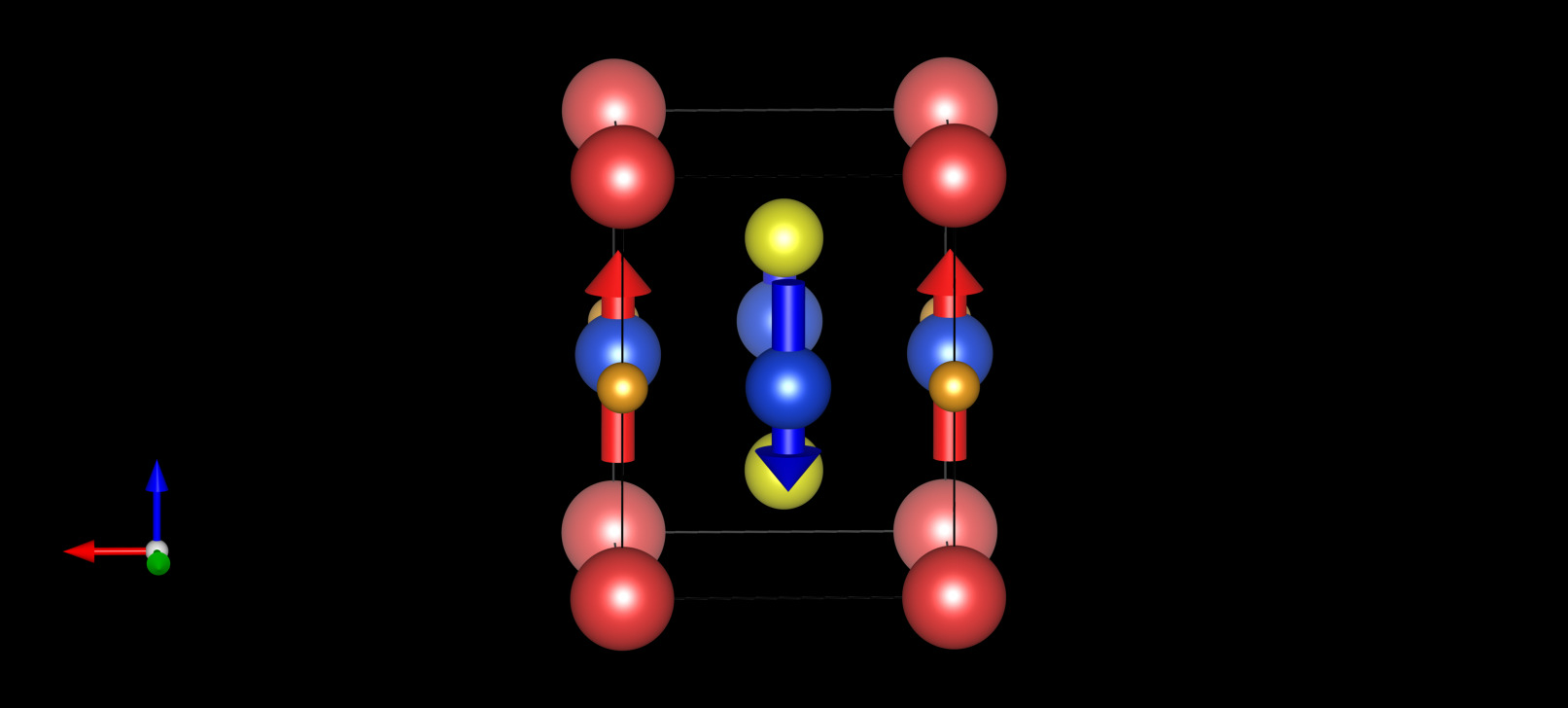
UCr 2 Si 2 C crystallizes in a tetragonal structure belonging to the paramagnetic space group P 4/mmm (No. 123), characterized by lattice parameters a = b = 3.98 and c = 5.16 [41]. The structure is composed of alternating uranium and Cr 2 Si 2 C layers stacked along the crystallographic c-axis. Within each Cr 2 Si 2 C layer, chromium atoms form planar Cr 2 C networks arranged in a checkerboard motif. Magnetic moments are localized exclusively on the Cr atoms, which occupy two
to align antiparallel, with an estimated magnitude of ap-
Under this collinear AFM configuration, UCr 2 Si 2 C is associated with the magnetic space group P m ′ m ′ m (No. 47.252, BNS notation), which determine its magnetic symmetry properties. This group comprises eight symmetry elements: four unitary operations that preserve spin namely, the identity {1 | 0}, spatial inversion
and a mirror reflection across the plane perpendicular to the x-axis {m 100 | 0} as well as four anti-unitary operations combining spatial transformations with timereversal symmetry. These include the twofold rotations about the z-axis combined with time reversal {2 ′ 001 | 0} and a twofold rotation about the y-axis combined with time reversal {2 ′ 010 | 0}, and the time-reversed mirror reflections {m ′ 001 | 0} and {m ′ 010 | 0}. These operations collectively preserve the overall tetragonal crystal symmetry while accommodating a collinear antiferromagnetic configuration with Cr.
Crucially, although both inversion P {−1 | 0} and antiunitary time revesal T = {−1 ′ | 0} symmetries appear in the group, the combined operation PT = {−1 ′ | 0} does not constitute a symmetry of the system. The absence of PT symmetry lifts the constraint that would otherwise enforce spin degeneracy, thereby permitting spin splitting even in the absence of spin–orbit coupling. Furthermore, the system lacks the combined spin-rotation and non-primitive lattice translation symmetry U τ , which maps antiparallel magnetic sublattices onto one another via a 180 ◦ spin rotation coupled with a fractional lattice translation. Such symmetries are characteristic of conventional collinear antiferromagnets and protect spin degeneracy throughout the Brillouin zone. In contrast, the symmetry-inequivalent positioning of the Cr atoms in UCr 2 Si 2 C precludes the existence of any U τ operation. The simultaneous breaking of both PT and U τ symmetries thus defines the altermagnetic nature of UCr 2 Si 2 C.
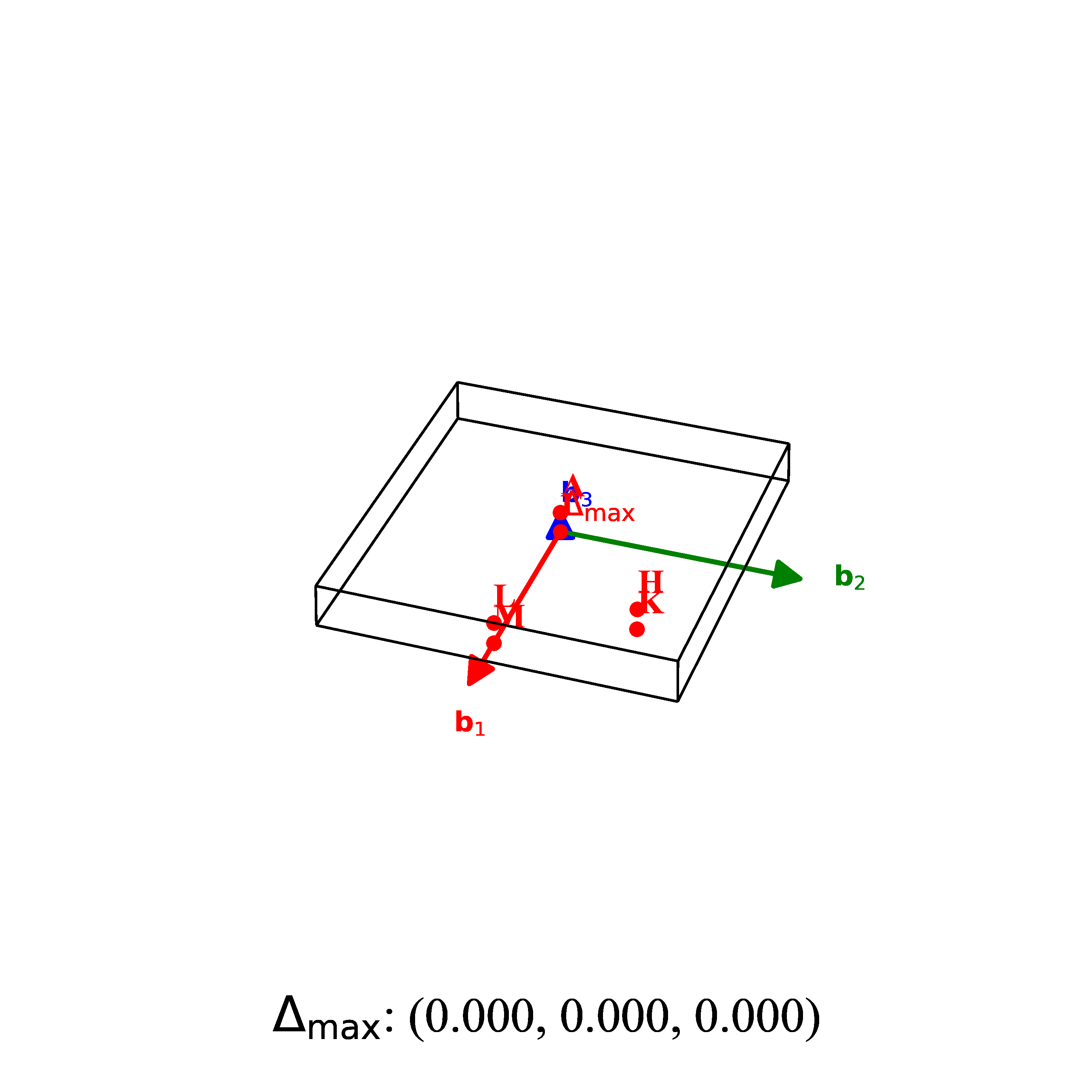
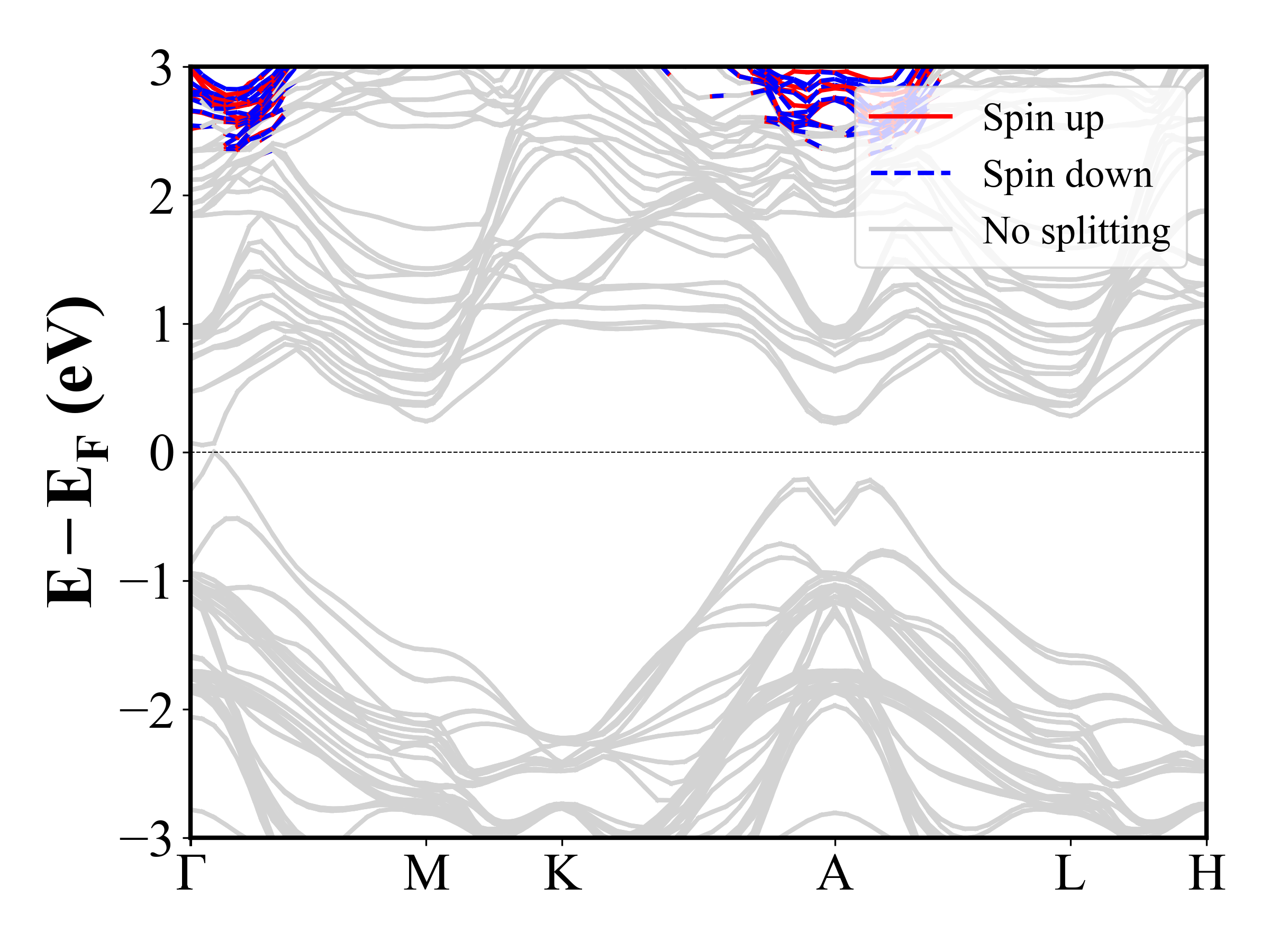
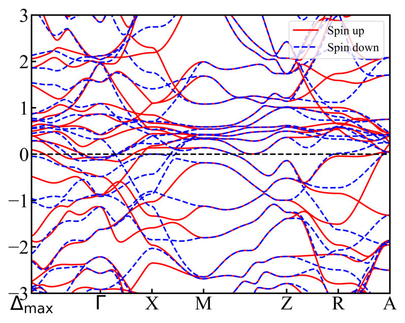
Figure 2(c) presents the spin-polarized electronic band structure of UCr 2 Si 2 C along high-symmetry paths in the Brillouin zone, as defined in Fig.2(b). Spin-up and spin-down states are shown in red and blue, respectively. A prominent feature of the band structure is the coexistence of spin-degenerate and spin-split regions across momentum space, hallmarks of altermagnetic behavior. The maximum energy separation occurs near the ∆ max point, where the spin splitting reaches approximately 0.72 eV. The average spin splitting across the Brillouin zone is calculated to be 0.31eV, with a volumetric splitting ratio of roughly 47%. To explicitly identify symmetry-driven spin reversals, we analyzed symmetryequivalent paths in the reciprocal space, as shown in panel (d). Specifically, along paths such as ∆ max –Γ– ∆ ′ max and R–A–R ′ , exchanging the reciprocal-space coordinates k x ↔ k y directly leads to inversion of the spin polarization (spin-up states become spin-down and vice versa). This momentum-dependent spin reversal arises naturally from the magnetic symmetry operations of the P m ′ m ′ m space group and it distinguishes altermagnetic systems from conventional ferromagnets or Rashba-type spin–orbit coupled systems.
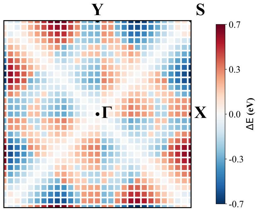
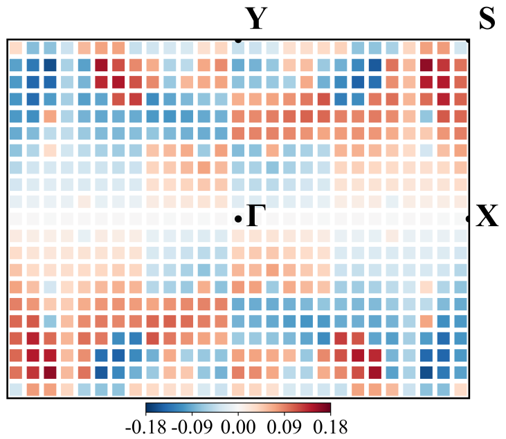
To further visualize the momentum-resolved spin splitting, we plot the two-dimensional (2D) contour map of the spin splitting magnitude (∆E) on the k z = 0.5 plane in Fig. 2(e). This plane includes the maximum splitting
splitting occurs. In this map, red and blue regions respectively indicate positive and negative spin splitting between spin-up and spin-down states. The most intense features appear in the vicinity of ∆ max , with symmetric but sign-reversed spin splitting observed on opposite sides of the Brillouin zone. This antisymmetric pattern
signature of altermagnetic order in this material.
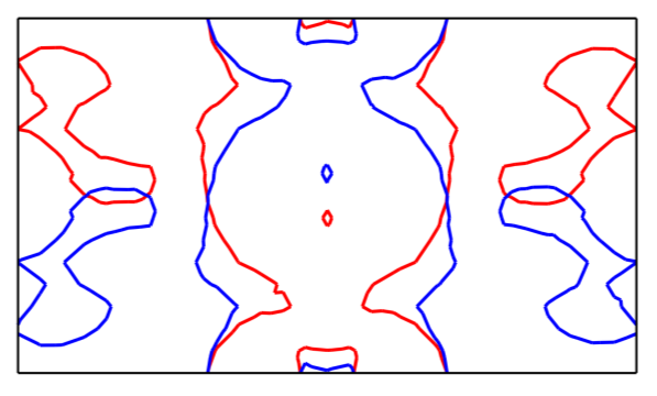
Figure 2(f) shows the spin-resolved Fermi surface crosssections in the (001) plane. Spin-up and spin-down Fermi
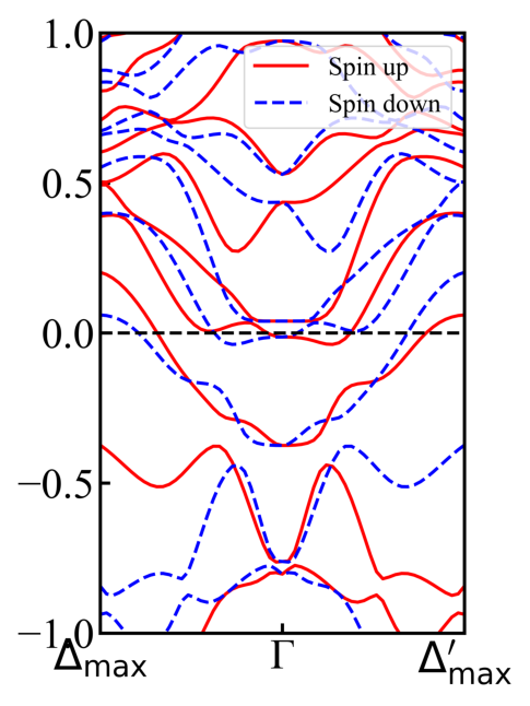
contours are shown in red and blue, respectively. The contours are anisotropic and exhibit a clear 90 ◦ rotation between the spin channels, another hallmark of altermagnetism. To fully capture the spin-dependent topology of the Fermi surface, we plot the three-dimensional spin-resolved Fermi surfaces in Figs. 2(g) and 2(h) for the spin-up and spin-down channels, respectively. Each plot reveals four distinct Fermi surfaces corresponding to four partially occupied bands crossing the Fermi level. Notably, while the innermost Fermi surface centered at the corners of the Brillouin zone appears nearly identical for both spin channels, the remaining three Fermi sheets (colored yellow, blue, and pink) exhibit clear rotational asymmetry. The spin-down Fermi surfaces are clearly rotated by 90 ◦ relative to their spin-up counterparts, consistent with the antisymmetric spin texture expected from the symmetry constraints of the magnetic space group. Together, these observations, momentumantisymmetric spin splitting, 90 ◦ -rotated spin-resolved Fermi surfaces, and symmetry-induced spin channel inversion, provide compelling evidence for the robust altermagnetic character of UCr 2 Si 2 C.
NbMnP crystallizes in the TiNiSi−type orthorhombic structure belonging to the paramagnetic space group Pnma (No. 62), characterized by lattice parameters
structure comprises zigzag chains of Mn atoms aligned along the b-axis, embedded within a network formed by Nb and P atoms. In this study, we consider a collinear AFM configuration as depicted in Fig. 3(a).
The magnetic symmetry properties of this AFM state are governed by magnetic space group P n ′ m ′ a ′ (No. 62.449, BNS notation), a type-III magnetic subgroup of the paramagnetic parent group Pnma (No. 62). This magnetic group incorporates eight symmetry elements: four unitary operations preserving spin specifically, the identity {1 | 0}, spatial inversion {−1 | 0}, mirror reflec-
cluding time-reversed inversion {−1 ′ | 12 , 0, 12 }, a time-
6
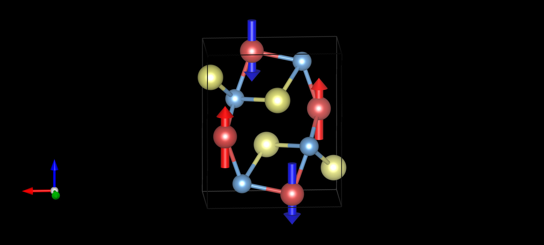
Critically, both PT and U τ symmetries are absent which implies that no symmetry exists to map the antiparallel Mn sublattices onto one another, thereby lifting the constraints that would typically enforce spin degeneracy in conventional antiferromagnets.
firm the altermagnetic character of NbMnP.
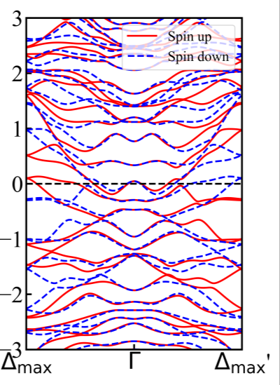
The spin-polarized electronic band structure along standard high-symmetry paths is presented in Fig. 3(c), with spin-up and spin-down channels shown in red and blue, respectively. Pronounced spin splitting regions coexist with segments of near degeneracy. The maximum spin splitting, approximately 0.46 eV, occurs near the ∆ max point, whereas the BZ-averaged splitting is about 0.28 eV with a volumetric splitting ratio of 35%. To illustrate symmetry-enforced spin reversal explicitly, Fig. 3(d) displays the spin-resolved bands along the path ∆ max –Γ–∆ ′ max , demonstrating symmetric spin-band exchange under the transformation k x → −k x across Γ.
YRuO 3 crystallizes in the orthorhombic magnetic space group P n ′ ma ′ (No. 62.448, BNS notation), derived from the paramagnetic parent group Pnma (No. 62) [43]. The unit cell adopts lattice parameters a = 5.839 Å,
described as a tilted perovskite framework composed of corner-sharing RuO 6 octahedra, with Y atoms occupying the interstitial positions. The magnetic ground state is G-type antiferromagnetic, with antiparallel spin alignment between neighboring Ru 3+ sites along all three crystallographic directions. The spin moments are localized on the Ru sublattices, whereas Y and O atoms remain magnetically inactive. Addtionally, it includes standard unitary operations, such as inversion, mirror planes, and twofold rotations, along with anti-unitary operations that combine time reversal with rotations and mirrors (e.g., 2 ′ 001 , m ′ 100 , m ′ 001 ). The resulting AFM structure consists of two symmetry-inequivalent Ru sublattices with antiparallel spin orientations. This arrangement prevents any symmetry operation from mapping one sublattice onto the other via inversion–time-reversal (PT ) or spinrotation–translation (Uτ ). This dual symmetry breaking allows for spin splitting even without spin–orbit couFigure 3(e) shows the spin-splitting magnitude ∆E within the k z = 0.25 plane, revealing clearly signreversed splitting distributions across opposite sides of the BZ. Additionally, Fig. 3(f) presents the spin-resolved Fermi surface cross-section at k z = 0.05, exhibiting distinctly anisotropic contours and a clear 180 ◦ rotation between the spin channels, consistent with k x ↔ −k x symmetry. The 3D spin-resolved Fermi surfaces shown in Figs. 3(g) and 3(h) for spin-up and spin-down channels, respectively, further highlight this 180 ◦ spin-channel rotation. Taken together, these observations robustly con-
7
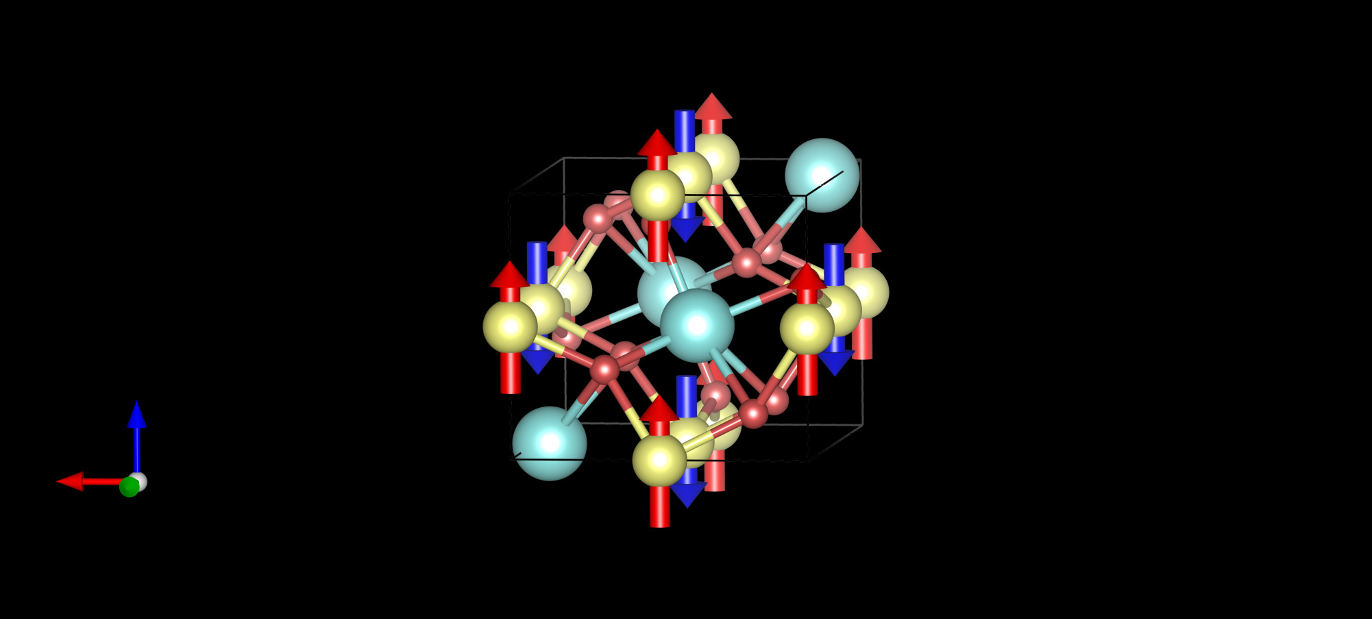
pling, which is what defines the altermagnetic nature of YRuO 3 .
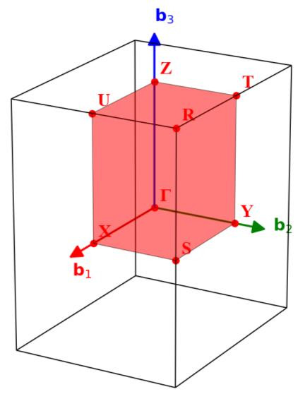
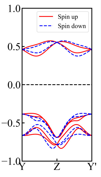
Figure 4(b) shows the bulk Brillouin zone BZ YRuO 3 with the high-symmetry points labeled according to the Pnma convention. The spin-polarized electronic band structure, computed along these high-symmetry paths, is presented in Fig. 4(c). A key feature is the coexistence of spin-degenerate and spin-split bands. The magnitude of spin splitting varies across momentum space, reaching its maximum near the ∆ max point, where the energy separation between spin-up and spin-down bands is approximately 0.12 eV.
To visualize the symmetry-driven spin inversion, Fig. 4(d) compares the band dispersions along two momentum paths that are equivalent under the transformation k x → −k x . Along these symmetry-related paths, the spin polarization reverses: spin-up states on the ∆ max /Y side correspond to spin-down states on the −∆ max /−Y side, reflecting the momentum-antisymmetric spin splitting enforced by the P n ′ ma ′ magnetic group. Figure 4(e) further highlights this feature through a 2D contour map of ∆E in the k z = 0.1 plane, where the splitting is maximal around ∆ max . Figure 4(f) illustrates the spin texture in the (001) plane from a SOC (noncollinear) calculation, showing the in-plane orientation of the spin expectation value for states near the Fermi level. The spin-up and spin-down components exhibit opposite orientations across symmetry-related k-points, indicating a momentum-dependent spin reversal that extends across the Brillouin zone rather than being localized to a specific path or point.
To identify bulk altermagnetic compounds with chemically equivalent 2D counterparts, we compared the reduced formulas and ICSD IDs of all 188 bulk AM candidates with entries in two major 2D materials databases: the Computational 2D Materials Database (C2DB) [44] and the AiiDA 2D repository [45]. We only retain entries for which the ICSD ID of the bulk parent coincides with that of the corresponding 2D record. In Table I, we collect all bulk AM materials whose reduced formula 8 TABLE I. Bulk altermagnetic materials with an existing 2D compound of the same reduced chemical formula in the C2DB or AiiDA databases. Multiple MCIF entries with identical formulas correspond to distinct MAGNDATA models. IDs 0.15 0.178, 0.334 0.335, 0.581, 1.0.33 0.36 0.607 0.800 1.0.47, 1.0.48 2.35 0.65, 0.66 Chemical formula
MnTe MnSe 2 CrSe Fe 2 O 3 C2DB Yes Yes Yes Yes Yes Yes Yes Yes – AiiDA
– – – – – – Yes – Yes appears in at least one of the 2D databases and indicate whether a match was found in C2DB, in AiiDA, or in both. These databases contain both experimentally synthesized and theoretically predicted monolayer compounds.
The list of bulk altermagnets with a corresponding two-dimensional compound is rather short. Indeed, the majority of compounds appearing in Table I contain transition–metal elements with partially filled d shells together with halogens (F, Cl) or chalcogens (S, Se, Te). The later help stabilizing layered or quasi-layered chemistries, while the former provide the local moments that form the basis of the magnetism.
Note that the first column of the table shows that some chemical formulas correspond to multiple MAGNDATA entries. The reason is that different experimental studies report distinct magnetic configurations, magnetic subgroup assignments, or slightly different crystallographic refinements. These duplicated entries correspond to separate magnetic models of the same material, not different compounds, and therefore belong match with a single two-dimensional material.
Table I identifies candidate bulk altermagnets which exist in 2D, but does not say that these materials are also altermagnetic as a monolayer. This question has been addressed by Sødequist and Olsen [46], who identified 7 altermagnetic monolayer candidates starting from C2DB. Crucially, they take into account the magnetic anisotropy coming from spin-orbit that is necessary to get a magnetically ordered phase in 2d, in accordance with the Mermin-Wagner theorem. Starting from C2DB, they identified which monolayers can be altermagnets, also taking into account spin-orbit coupling. The spin-orbit coupling introduces magnetic anisotropy that makes it possible to stabilize magnetism in 2d while satisfying the Mermin-Wagner theorem. Their 7 altermagnetic monolayer candidates similarly contain mostly transition metals terminated by halogens or chalcogens, although they also find two more complex compounds. Interestingly, there is zero overlap between Table I and the list in Sødequist and Olsen.
The results reported here can be discussed in relation to two prior screenings of MAGNDATA. The highthroughput classification by Wan et al. relied on the absence of the antiunitary symmetries PT (inversion plus time reversal) and tT (translation plus time reversal) [27]. Moreover, they extended their candidate pool to include ferrimagnetic systems by considering their SOC-off configuration, resulting in 336 potential altermagnets. Guo et al. also focused on systems with PT symmetry [29]. They screened stoichiometric compounds with fully compensated collinear magnetic order without ferromagnetic component while avoiding some complications, including systems with magnetic order from rare-earth atoms, large unit cells, and DFT calculations difficult to converge, which resulted in 62 materials.
Our study employs the amcheck algorithm, which tests the same symmetry condition (absence of PT and tT ) to identify potential altermagnetic materials. However, amcheck strictly excludes ferrimagnetic states since their sublattices are completely not symmetry-related and are instead classified as “Luttinger ferrimagnets” that exhibit spin splitting but lack the required momentumodd, nodal spin texture over the Brillouin zone. For example, Cr 2 S 3 , listed as “interesting” in Ref. [27], shows spin splitting in the spin–polarized DFT consistent with ferrimagnetic behavior, yet lacks the nodal spin texture and is therefore not classified as altermagnetic here. On the other hand, we find a collinear AFM with Kramers–degenerate bands for SrMnSb 2 , and the small splittings of a few meV that appear at high energy are most likely numerical artifacts and not indicative of altermagnetism. These distinctions likely account for the smaller number of altermagnets identified in our study compared to Ref. [27], while remaining fully consistent with the symmetry–based definition of altermagnetism [1, 2]. The 59 non-metallic and 3 metallic compounds identified in Ref. [29] all appear in our list of 157 collinear entries with the right symmetries for altermagnetism (see table S2 in the supplementary materials), however, the criterion of a spin splitting threshold of 26 meV for our final list removes 10 of them.
Furthermore, we have considered a set of collinear versions of materials reported as noncollinear. This extended set of materials along with their computed spin splittings describe alternative spin configurations on otherwise stable crystal structures. They can be a valuable resource to aid the general understanding of altermagnetism. Some of them are arguably relevant due to them being very nearly collinear, shown in our analysis by the angle between the spin axes. We also speculate that for some of the ones with larger such angles, there could exist ways in practice to invoke a more aligned moments to give the altermagnetic configuration, via, e.g., external fields, stress/strain, or similar mechanisms.
9 TABLE II. Top altermagnet candidate materials with respect to their spin-splitting. Space group, max angle between spins for materials that were originally noncollinear (arccos(|S i · S j |/|S i ||S j |)), spin-splitting metrics, band gap, wave classification, Hubbard U , and minimum elemental abundance. For more information on symmetry data, refer to the supplementary materials. |S ·S | Material Space Group
i
j
In this work, we have established a comprehensive and symmetry-aware high-throughput framework for the discovery and characterization of altermagnetic materials. We systematically screened more than 2,000 experimentally verified magnetic structures from the MAGNDATA database using a two-stage workflow. This approach, built on the magnetic symmetry diagnostic tool amcheck and the High-Throughput Toolkit, identified 180 candidate materials exhibiting significant momentumdependent spin splitting. These include both metallic and semiconducting systems, many of which had not been previously reported as altermagnets. Notably, our approach recovers experimentally confirmed compounds such as CrSb, MnTe, and RuO 2 , and highlights previously overlooked materials like UCr 2 Si 2 C, MnNbP, and YRuO 3 that display robust symmetry-protected spin splitting even in the absence of spin–orbit coupling. Furthermore, by cross-referencing our bulk AM candidates with the C2DB and AiiDA 2D repository, we identify nine materials with chemically equivalent 2D counterparts.
Crucially, our momentum-resolved analysis reveals that spin splitting varies strongly across the Brillouin zone, often away from high-symmetry paths, providing actionable insights for future spin and angle-resolved photoemission spectroscopy (ARPES) measurements. The open-access database generated through this effort offers a valuable resource for guiding experimental exploration and materials design in spintronics. More broadly, this study establishes a scalable and transferable blueprint for accelerating the discovery of unconventional magnetic phases and paves the way for targeted development of altermagnetic materials with desirable symmetry and transport properties.
This work was partially supported by the Wallenberg Initiative Materials Science for Sustainability (WISE) funded by the Knut and Alice Wallenberg Foundation. R.A. acknowledges financial support from the Swedish e-Science Research Centre (SeRC). EvL acknowledges support from the Swedish Research Council (Vetenskapsrådet, VR) under grant 2022-03090, from the Royal Physiographic Society in Lund and by eSSENCE, a strategic research area for e-Science, grant number eSSENCE@LU 9:1. J.A.L thank the Kempe-stiftelserna, Sweden and Swedish Research Council under grant no. 2023-03894 for financial support. B.M. acknowledge the financial support of Olle Engkvists stiftelse, project 207- 10 0582. The computations were enabled by resources provided by the National Academic Infrastructure for Supercomputing in Sweden (NAISS), partially funded by the Swedish Research Council through grant agreement no. 2022-06725.
Appendix A: Computational Details Density functional theory (DFT) calculations were carried out using the Vienna Ab initio Simulation Package (VASP) [37, 38], employing the projector augmentedwave (PAW) method and the generalized gradient approximation (GGA) with the Perdew–Burke–Ernzerhof (PBE) functional to describe exchange-correlation effects [36, 47]. Electron correlation was treated using the rotationally invariant DFT+U approach [48], with the effective Hubbard U eff parameters taken from Pymatgen (Materials Project) [49] and supplemented by Wang et al. [50] where needed. The magnitude of the spin splitting depends on the value of U via the magnitude of the magnetic moments [51], whereas the structure of the splitting in the Brillouin Zone is expected to be weakly dependent on the value of U . Consistent with this, recalculations with U scaled by ±10% for all metallic candidates show that the altermagnetic classification is unchanged and sizable splittings persist; the variations are mainly quan[1] L. Šmejkal, J. Sinova, and T. Jungwirth, Beyond conven-
tional ferromagnetism and antiferromagnetism: A phase with nonrelativistic spin and crystal rotation symmetry, Physical Review X 12, 031042 (2022). [2] L. Šmejkal, J. Sinova, and T. Jungwirth, Emerging re-
search landscape of altermagnetism, Physical Review X 12, 040501 (2022). [3] I. Mazin and PRX editors, Altermagnetism—a new
punch line of fundamental magnetism (2022). [4] K.-H. Ahn, A. Hariki, K.-W. Lee, and J. Kuneš, Antifer-
romagnetism in RuO2 as d-wave Pomeranchuk instability, Physical Review B 99, 184432 (2019). [5] M. Naka, S. Hayami, H. Kusunose, Y. Yanagi, Y. Mo-
tome, and H. Seo, Spin current generation in organic antiferromagnets, Nature communications 10, 4305 (2019). [6] L. Šmejkal, R. González-Hernández, T. Jungwirth, and
spontaneous hall effect in collinear antiferromagnets, Science advances 6, eaaz8809 (2020). [7] L.-D. Yuan, Z. Wang, J.-W. Luo, E. I. Rashba, and
in centrosymmetric low-z antiferromagnets, Physical Review B 102, 014422 (2020). [8] S. Hayami, Y. Yanagi, and H. Kusunose, Bottom-up de-
sign of spin-split and reshaped electronic band structures in antiferromagnets without spin-orbit coupling: Procedure on the basis of augmented multipoles, Physical Review B 102, 144441 (2020). [9] H.-Y. Ma, M. Hu, N. Li, J. Liu, W. Yao, J.-F. Jia, and
J. Liu, Multifunctional antiferromagnetic materials with titative and not strictly monotonic, with only Co 2 Mo 3 O 8 turning insulating at U +10% (Table S4).
For all simulations, the plane-wave energy cutoff was automatically set to 1.3 times the maximum ENMAX value among the elements present in the system, following VASP’s recommended settings and the electronic self-consistency loop was converged to within 10 −6 eV. K-point meshes for SCF calculations were automatically generated by Pymatgen, targeting a density of approximately 1000 k-points per reciprocal atom. For NSCF calculations, the k-point mesh was manually doubled along each reciprocal axis to ensure accurate Brillouin zone sampling for spin-splitting analysis. Although canted magnetic configurations occur in many materials, for computational efficiency we approximated their magnetic structures using collinear spin arrangements to identify signatures of altermagnetism.
High-throughput calculations were managed using httk [35]. High-symmetry k-paths were constructed using Pymatgen [34], and magnetic space groups were identified using the Spglib library [32, 33]. Fermi surfaces and spin textures were visualized using the IFermi package [52].
The elemental abundance values, expressed in parts per million (ppm) with respect to the Earth’s crust, were obtained using the mendeleev [53] Python library and are reported in the table.
giant piezomagnetism and noncollinear spin current, Nature communications 12, 2846 (2021). [10] I. I. Mazin, K. Koepernik, M. D. Johannes, R. González-
Hernández, and L. Šmejkal, Prediction of unconventional magnetism in doped FeSb2, Proceedings of the National Academy of Sciences 118, e2108924118 (2021). [11] P. Liu, J. Li, J. Han, X. Wan, and Q. Liu, Spin-group
symmetry in magnetic materials with negligible spinorbit coupling, Physical Review X 12, 021016 (2022). [12] S. Rooj, S. Saxena, and N. Ganguli, Altermagnetism in
the orthorhombic P nma structure through group theory and DFT calculations, Physical Review B 111, 014434 (2025). [13] S. Hayami, Y. Yanagi, and H. Kusunose, Momentum-
dependent spin splitting by collinear antiferromagnetic ordering, journal of the physical society of japan 88, 123702 (2019). [14] J. Krempaskỳ, L. Šmejkal, S. D’souza, M. Hajlaoui,
G. Springholz, K. Uhlířová, F. Alarab, P. Constantinou,
kramers spin degeneracy, Nature 626, 517 (2024). [15] C.-C. Wei, E. Lawrence, A. Tran, and H. Ji, Crystal
chemistry and design principles of altermagnets, ACS Organic & Inorganic Au 4, 604 (2024). [16] O. Fedchenko, J. Minár, A. Akashdeep, S. W. D’Souza,
D. Vasilyev, O. Tkach, L. Odenbreit, Q. Nguyen, D. Kutnyakhov, N. Wind, et al., Observation of time-reversal symmetry breaking in the band structure of altermagnetic ruo2, Science advances 10, eadj4883 (2024). [17] H. Reichlova, R. Lopes Seeger, R. González-Hernández,
11
mel, M. Leiviskä, A. Birk Hellenes, et al., Observation of a spontaneous anomalous Hall response in the Mn5Si3 d-wave altermagnet candidate, Nature Communications 15, 4961 (2024). [18] S. Reimers, L. Odenbreit, L. Šmejkal, V. N. Strocov,
P. Constantinou, A. B. Hellenes, R. Jaeschke Ubiergo, W. H. Campos, V. K. Bharadwaj, A. Chakraborty, et al., Direct observation of altermagnetic band splitting in CrSb thin films, Nature Communications 15, 2116 (2024). [19] L. Šmejkal, A. H. MacDonald, J. Sinova, S. Nakatsuji,
and T. Jungwirth, Anomalous Hall antiferromagnets, Nature Reviews Materials 7, 482 (2022). [20] R. Gonzalez Betancourt, J. Zubáč, R. Gonzalez-
Hernandez, K. Geishendorf, Z. Šobáň, G. Springholz, K. Olejník, L. Šmejkal, J. Sinova, T. Jungwirth, et al., Spontaneous anomalous Hall effect arising from an unconventional compensated magnetic phase in a semiconductor, Physical Review Letters 130, 036702 (2023). [21] L. Šmejkal, A. B. Hellenes, R. González-Hernández,
J. Sinova, and T. Jungwirth, Giant and tunneling magnetoresistance in unconventional collinear antiferromagnets with nonrelativistic spin-momentum coupling, Physical Review X 12, 011028 (2022). [22] R. González-Hernández, L. Šmejkal, K. Vỳbornỳ, Y. Ya-
hagi, J. Sinova, T. Jungwirth, and J. Železnỳ, Efficient electrical spin splitter based on nonrelativistic collinear antiferromagnetism, Physical Review Letters 126, 127701 (2021). [23] H. Bai, Y. Zhang, Y. Zhou, P. Chen, C. Wan, L. Han,
W. Zhu, S. Liang, Y. Su, X. Han, et al., Efficient spin-tocharge conversion via altermagnetic spin splitting effect in antiferromagnet RuO2, Physical review letters 130, 216701 (2023). [24] A. Bose, N. J. Schreiber, R. Jain, D.-F. Shao, H. P.
Nair, J. Sun, X. S. Zhang, D. A. Muller, E. Y. Tsymbal, D. G. Schlom, et al., Tilted spin current generated by the collinear antiferromagnet ruthenium dioxide, Nature Electronics 5, 267 (2022). [25] S. V. Gallego, J. M. Perez-Mato, L. Elcoro, E. S.
Tasci, R. M. Hanson, K. Momma, M. I. Aroyo, and
netic structures. I. the commensurate case, Journal of Applied Crystallography 49, 1750–1776 (2016). [26] S. V. Gallego, J. M. Perez-Mato, L. Elcoro, E. S. Tasci,
data: towards a database of magnetic structures. ii. the incommensurate case, Applied Crystallography 49, 1941 (2016). [27] X. Wan, S. Mandal, Y. Guo, and K. Haule, High-
throughput search for metallic altermagnets by embedded dynamical mean field theory, arXiv preprint arXiv:2412.10356 (2024). [28] X. Chen, Y. Liu, P. Liu, Y. Yu, J. Ren, J. Li, A. Zhang,
and Q. Liu, Unconventional magnons in collinear magnets dictated by spin space groups, Nature , 1 (2025). [29] Y. Guo, H. Liu, O. Janson, I. C. Fulga, J. van den Brink,
and J. I. Facio, Spin-split collinear antiferromagnets: A large-scale ab-initio study, Materials Today Physics 32, 100991 (2023). [30] M. I. Aroyo, J. M. Perez-Mato, C. Capillas, and H. Won-
dratschek, The Bilbao crystallographic server, in International Tables for Crystallography (International Union of Crystallography, 2011) p. 57–69. [31] A. Smolyanyuk, L. Šmejkal, and I. I. Mazin, A tool
to check whether a symmetry-compensated collinear magnetic material is antiferro-or altermagnetic, SciPost Physics Codebases , 030 (2024). [32] K. S. Atsushi Togo and I. Tanaka, Spglib: a software
library for crystal symmetry search, Sci. Technol. Adv. Mater., Meth. 4, 2384822 (2024). [33] K. Shinohara, A. Togo, and I. Tanaka, Algorithms for
magnetic symmetry operation search and identification of magnetic space group from magnetic crystal structure, Acta Cryst. A 79, 390 (2023). [34] S. P. Ong, W. D. Richards, A. Jain, G. Hautier,
M. Kocher, S. Cholia, D. Gunter, V. L. Chevrier, K. A. Persson, and G. Ceder, Python materials genomics (pymatgen): A robust, open-source python library for materials analysis, Computational Materials Science 68, 314 (2013). [35] R. Armiento, B. Kozinsky, G. Pizzi, et al., High-
throughput toolkit (httk), https://httk.org/ (2016), python package for high-throughput calculations. [36] P. E. Blöchl, Projector augmented-wave method, Phys.
Rev. B 50, 17953 (1994). [37] G. Kresse and J. Furthmüller, Efficient iterative schemes
for ab initio total-energy calculations using a plane-wave basis set, Phys. Rev. B 54, 11169 (1996). [38] G. Kresse and D. Joubert, From ultrasoft pseudopoten-
tials to the projector augmented-wave method, Phys. Rev. B 59, 1758 (1999). [39] S. Picozzi, Spin–orbit coupling in quantum materials:
Emergent phenomena, their modelling and examples from 2d magnets, EPJ Quantum Technology 12, 1 (2025). [40] Z. Liu, M. Ozeki, S. Asai, S. Itoh, and T. Masuda, Chi-
ral split magnon in altermagnetic mnte, Physical Review Letters 133, 156702 (2024). [41] P. Lemoine, A. Verniere, M. Pasturel, G. Venturini, and
substructure in UCr2Si2C and structural relationships in quaternary U-Cr-Si-C compounds, Inorganic Chemistry 57, 2546 (2018). [42] M. Matsuda, D. Zhang, Y. Kuwata, Q. Zhang, T. Saku-
rai, H. Ohta, H. Sugawara, K. Takeda, J. Hayashi, and H. Kotegawa, Noncollinear spin structure with weak ferromagnetism in nbmnp, Physical Review B 104, 174413 (2021). [43] K. Ji, A. Paul, E. Solana-Madruga, A. M. Arevalo-Lopez,
weak ferromagnet, Physical Review Materials 4, 091402 (2020). [44] S. Haastrup, M. Strange, M. Pandey, T. Deilmann,
sen, The computational 2d materials database: highthroughput modeling and discovery of atomically thin crystals, 2D Materials 5, 042002 (2018). [45] G. Pizzi, A. Cepellotti, R. Sabatini, N. Marzari, and
B. Kozinsky, Aiida: automated interactive infrastructure and database for computational science, Computational Materials Science 111, 218 (2016). [46] J. Sødequist and T. Olsen, Two-dimensional altermag-
nets from high throughput computational screening: Symmetry requirements, chiral magnons, and spin-orbit effects, Applied Physics Letters 124, 182409 (2024). [47] J. P. Perdew, K. Burke, and M. Ernzerhof, Generalized 12 gradient approximation made simple, Physical review letters 77, 3865 (1996). [48] V. I. Anisimov, J. Zaanen, and O. K. Andersen, Band
theory and Mott insulators: Hubbard U instead of Stoner I, Physical Review B 44, 943 (1991). [49] A. Jain, S. P. Ong, G. Hautier, et al., Commentary: The
materials project: A materials genome approach to accelerating materials innovation, APL Materials 1, 011002 (2013). [50] L. Wang, T. Maxisch, and G. Ceder, Oxidation energies
of transition metal oxides within the GGA+U framework, Physical Review B 73, 195107 (2006). [51] M. Roig, A. Kreisel, Y. Yu, B. M. Andersen, and D. F.
Agterberg, Minimal models for altermagnetism, Phys. Rev. B 110, 144412 (2024). [52] A. M. Ganose, A. Searle, A. Jain, and S. M. Griffin,
IFermi: A python library for Fermi surface generation and analysis, Journal of Open Source Software 6, 3089 (2021). [53] Łukasz Mentel, mendeleev: A python resource for prop-
erties of chemical elements, ions and isotopes, https: //pypi.org/project/mendeleev/ (2014).
Ali Sufyan, 1,2,3 Brahim Marfoua, 4 J. Andreas Larsson, 3,5 Erik van Loon, 1,2 and Rickard Armiento 4 2 1 NanoLund and Division of Mathematical Physics, Department of Physics, Lund University, SE-221 00 Lund, Sweden Wallenberg Initiative Materials Science for Sustainability, Department of Physics, Lund University, SE-221 00 Lund, Sweden 3 Applied Physics, Division of Materials Science, Department of Engineering Sciences and Mathematics, Luleå University of
Technology, SE-971 87 Luleå, Sweden 4 Department of Physics, Chemistry and Biology, Linköping University, SE-581 83 Linköping, Sweden 5 Wallenberg Initiative Materials Science for Sustainability, Luleå University of Technology, SE-971 87 Luleå, Sweden Table S1: High-throughput screening results for candidate altermagnets. The table lists the MAGNDATA ID(s), material, space group, spin-splitting metrics (F ∆ , Max SS, Avg SS), band gap, and minimum elemental crustal abundance, and is ordered by decreasing Max SS. When multiple MAGNDATA IDs are listed for the same material/space group, the first ID corresponds to the record with the largest Max SS and the values reported in the remaining columns, while the other listed IDs are also identified as altermagnets with Max SS > 26 meV.
| MAGNDATA ID Material | Space group F ∆ (%) Max SS Avg SS Bandgap Min abund. (ppm) |
|---|---|
| 0.528 CrSb | P63 /mmc 34.375 1.872 0.763 0.000 2.000 × 10⁻¹ |
| 0.8 MnTe | P63 /mmc 34.375 0.923 0.449 0.764 1.000 × 10⁻³ |
| 0.607 RuO2 | P42 /mnm 25.000 0.865 0.351 0.000 1.000 × 10⁻³ |
| 2.35 CrSe | P63 /mmc 35.938 0.800 0.489 0.000 5.000 × 10⁻² |
| 0.499 UCr2 Si2 C | P4/mmm 46.875 0.719 0.312 0.000 2.700 |
| 0.236 Ca(Al2 Fe)4 | I4/mmm 37.500 0.628 0.374 0.000 4.150 × 10⁴ |
| 0.296, 0.295 Cu2 O3 Cl | P21 /c 35.417 0.553 0.233 0.000 6.000 × 101 |
| 0.178 CoF2 | P42 /mnm 16.667 0.479 0.223 3.306 2.500 × 101 |
| 0.803 MnNbP | Pnma 35.000 0.457 0.276 0.000 2.000 × 101 |
| 0.36 NiF2 | P42 /mnm 27.083 0.392 0.180 5.268 8.400 × 101 |
| 0.131 Mn(C2 N3 )2 | Pnnm 16.250 0.348 0.156 3.742 1.900 × 101 |
| 0.501 LiFe2 F6 | P42 /mnm 12.500 0.319 0.159 0.168 2.000 × 101 |
| 0.1065 MnGeN2 | Pna21 14.583 0.305 0.145 1.516 1.500 |
| 0.113 NiCO3 | R-3c 20.833 0.301 0.167 4.197 8.400 × 101 |
| 0.128 FeSO4 F | C2/c 28.906 0.301 0.158 2.451 3.500 × 10² |
| 0.15 MnF2 | P42 /mnm 18.750 0.294 0.156 3.575 5.850 × 10² |
| 1.522 CrVO4 | Cmcm 28.571 0.292 0.158 2.877 1.020 × 10² |
| 0.402 Sr4 Fe4 O11 | Cmmm 29.808 0.289 0.150 0.176 3.700 × 10² |
| 0.99, 0.991, HoFeO3 | Pnma 25.893 0.283 0.126 2.835 1.300 |
| 0.992, 0.993, | |
| 0.994 | |
| 0.375 La2 CoIrO6 | P21 /c 24.107 0.272 0.121 0.000 1.000 × 10⁻³ |
| 0.351 TbFeO3 | Pnma 26.786 0.271 0.133 2.826 1.200 |
| 0.813, 0.81, Fe2 WO6 | Pbcn 29.688 0.270 0.173 1.465 1.250 |
| 0.811, 0.812 | |
| 0.154 Er2 Ru2 O7 | Fd-3m 20.313 0.268 0.266 0.412 1.000 × 10⁻³ |
| 0.112 FeBO3 | R-3c 29.688 0.262 0.177 2.660 1.000 × 101 |
| 0.837, 0.836, DyFeO3 | Pnma 26.786 0.261 0.134 2.863 5.200 |
| 0.841, 0.84, | |
| 0.838, 0.839, | |
| 0.1, 0.11 | |
| 0.309 TlCrO3 | Pnma 24.107 0.246 0.146 0.625 8.500 × 10⁻¹ |
| 0.1049 CoH6 (CO3 )2 | P21 /c 14.773 0.245 0.132 1.908 2.500 × 101 |
| 0.1067, 0.1066 MnSiN2 | Pna21 18.750 0.245 0.114 2.733 1.900 × 101 |
| 0.76 FeHSO5 | C2/c 26.563 0.242 0.156 2.625 3.500 × 10² |
| 0.103, 0.101, Mn2 GeO4 | Pnma 23.125 0.239 0.127 0.594 1.500 |
| 0.102 | |
| 0.66, 0.65 Fe2 O3 | R-3c 28.977 0.237 0.152 2.566 5.630 × 10⁴ |
| 0.59, 0.591 ErCrO3 | Pnma 21.875 0.234 0.108 3.143 3.500 |
| 0.308 CrInO3 | Pnma 20.536 0.232 0.132 1.886 2.500 × 10⁻¹ |
| 0.758, 0.759, CeFeO3 | Pnma 27.679 0.227 0.121 2.818 6.650 × 101 |
| 0.757 | |
| 0.307 ScCrO3 | Pnma 20.536 0.227 0.127 2.987 2.200 × 101 |
| 0.475 Sr2 TbIrO6 | P21 /c 27.083 0.226 0.114 0.139 1.000 × 10⁻³ |
| 0.698, 0.697 SmCrO3 | Pnma 20.536 0.222 0.095 3.115 7.050 |
| 0.586, 0.947 YCrO3 | Pnma 21.429 0.221 0.115 3.121 3.300 × 101 |
| 0.379 SmFeO3 | Pnma 27.679 0.215 0.124 2.843 7.050 |
| 0.261 FeNiPO5 | Pnma 24.375 0.207 0.121 2.694 8.400 × 101 |
| continued on next page |
La 2 CoIrO 6 TbFeO 3 Fe 2 WO 6 P2 1 /c Pnma Pbcn 24.107 26.786 29.688 0.272 0.271 0.270 0.121 0.133 0.173 0.000 2.826 1.465
1.200 1.250
Er 2 Ru 2 O 7 FeBO 3 DyFeO 3 Fd-3m R-3c Pnma 20.313 29.688 26.786 0.268 0.262 0.261 0.266 0.177 0.134 0.412 2.660 2.863
5.200 TlCrO 3 CoH 6 (CO 3 ) 2 MnSiN 2 FeHSO 5 Mn 2 GeO 4 Pnma P2 1 /c Pna2 1 C2/c Pnma 24.107 14.773 18.750 26.563 23.125 0.246 0.245 0.245 0.242 0.239 0.146 0.132 0.114 0.156 0.127 0.625 1.908 2.733 2.625 0.594
Fe 2 O 3 ErCrO 3 CrInO 3 CeFeO 3 R-3c Pnma Pnma Pnma 28.977 21.875 20.536 27.679 0.237 0.234 0.232 0.227 0.152 0.108 0.132 0.121 2.566 3.143 1.886 2.818
3.500
ScCrO 3 Sr 2 TbIrO 6 SmCrO 3 YCrO 3 SmFeO 3 FeNiPO 5 Pnma P2 1 /c Pnma Pnma Pnma Pnma 20.536 27.083 20.536 21.429 27.679 24.375 0.227 0.226 0.222 0.221 0.215 0.207 0.127 0.114 0.095 0.115 0.124 0.121 2.987 0.139 3.115 3.121 2.843 2.694
7.050
7.050
continued on next page 1 Table S1 (continued). MAGNDATA ID Material Space group F ∆ (%) Max SS Avg SS Bandgap Min abund. (ppm) 0.609, 0.288, 0.37 0.592, 2.64, 2.63 0.587 0.983, 0.982 0.392 0.1085 0.26 0.25 0.336, 0.337 0.1071 0.642, 0.1 0.354, 2.62 0.114 0.1021, 0.1022 0.295 0.896 0.315 0.323, 0.417 1.0.47 0.608 0.298 0.5 0.21 0.314 0.788 0.792, 0.794, 0.793 0.589 0.105, 0.104 0.262 0.115 0.712 1.0.33 0.714 0.1068 0.116 0.747 0.334 0.937, 0.301 0.1036 0.575 0.984 1.0.26 0.189 0.6 0.204 0.218, 0.219 0.148 0.755 0.581, 0.335 0.722 0.681 0.79 NdMnO 3 Pnma 19.643 0.206 0.143 1.420 4.150 × 10 1
DyCrO 3 Pnma 20.833 0.206 0.103 3.079 5.200
TmCrO 3 TmVO 3 Fe 3 P 2 (HO 5 ) 2 PrFeO 3 CuFePO 5 NaOsO 3 NdFeO 3 Fe 2 SiO 4 LaMnO 3 TbCrO 3 CoCO 3 TmFeO 3 Cu 2 H 3 ClO 3 CrNiO 4 ZrMn 2 (GeO 3 ) 4 LaCrO 3 MnSe 2 PrMnO 3 BaNa 2 V 2 FeO 8 TiMnO 3 NiPbO 3 ZrCo 2 (GeO 3 ) 4 YVO 3 Sr 2 HoRuO 6 Pnma P2 1 /c P2 1 /c Pnma Pnma Pnma Pnma Pnma Pnma Pnma R-3c Pnma P2 1 /c Cmcm P4/nbm Pnma Pa-3 Pnma C2/c R3c R3c P4/nbm P2 1 /c P2 1 /c 25.000 18.750 23.611 28.571 27.500 22.917 27.679 17.361 20.536 23.958 25.000 22.321 23.125 31.250 14.423 20.536 45.833 21.429 20.956 25.000 26.136 17.788 20.833 22.321 0.202 0.200 0.197 0.197 0.194 0.193 0.192 0.192 0.188 0.188 0.188 0.188 0.186 0.186 0.184 0.182 0.178 0.176 0.174 0.173 0.170 0.170 0.168 0.166 0.117 0.100 0.126 0.120 0.119 0.082 0.122 0.132 0.106 0.098 0.125 0.124 0.055 0.109 0.105 0.097 0.133 0.107 0.102 0.101 0.111 0.110 0.067 0.084 3.141 1.739 2.051 2.822 1.955 0.119 2.833 2.940 1.283 3.114 2.766 0.762 1.749 2.000 2.309 3.105 0.983 0.896 2.710 2.470 0.561 2.628 2.043 1.031
NdCrO 3 ErVO 3 CoFePO 5 MnCO 3 Nb 3 VS 6 FeF 3 Li 2 Ni(SO 4 ) 2 LuCrO 3 FeCO 3 Ba 3 CoIr 2 O 9 CoF 3 Sr 2 CoTeO 6 CoTa 4 Se 8 ZnFeH 4 O 2 F 5 LuVO 3 RbCoBr 3 CeMn 2 Ge 4 O 12 YMnO 3 Ca 2 MnReO 6 Co 2 SiO 4 LiLa 2 RuO 6 Mn 2 SeO 3 F 2 FeF 3 Mn 4 Nb 2 O 9 Ce 4 Sb 3 Sr 2 DyRuO 6 Pnma Pnma Pnma R-3c P6 322 P6 3 /m P2 1 /c Pnma R-3c C2/c R-3c P2 1 /c P6 3 /mmc Imm2 Pnma P6 3 /mmc P4/nbm P6 3 cm P2 1 /c Pnma P2 1 /c Pnma R-3c Cc I-43d P2 1 /c 19.643 18.750 26.875 19.531 31.250 31.250 20.536 19.792 17.361 29.167 31.250 29.167 36.719 23.438 18.750 24.432 18.269 21.875 11.458 22.222 26.042 21.250 32.813 21.250 47.500 23.214 0.165 0.165 0.164 0.161 0.161 0.159 0.158 0.158 0.157 0.156 0.155 0.155 0.154 0.154 0.153 0.150 0.149 0.145 0.145 0.144 0.142 0.141 0.141 0.140 0.139 0.138 0.107 0.082 0.103 0.112 0.057 0.080 0.077 0.125 0.110 0.124 0.095 0.088 0.126 0.074 0.073 0.100 0.117 0.092 0.076 0.101 0.093 0.095 0.094 0.078 0.058 0.081 3.079 1.971 2.399 4.015 0.000 3.764 4.565 3.192 3.688
1.825 2.154 0.000 3.124 1.991 0.000 0.000 1.305 0.000 2.506 1.221 3.889 4.342 1.270 0.000 1.114
continued on next page 2
Table S1 (continued). MAGNDATA ID Material Space group F ∆ (%) Max SS Avg SS Bandgap Min abund. (ppm) 0.513 0.121 0.83 0.1008 0.795 0.263 0.31, 0.32, 0.33 0.98, 0.981, 0.979 0.999, 0.1 0.1059 0.117 0.67, 0.669 0.671 0.24 3.4 0.241 0.416 0.791 0.168 0.45 0.787 0.948 0.934 0.42 0.122 0.108 0.708 0.165 0.7, 0.8 0.582, 2.61 0.802 0.1082 0.748 0.192 1.0.39 0.936 0.368 0.41, 0.40 0.294 0.229 0.79 0.1018, 0.1019 0.967 0.292 0.917 0.785, 0.786 0.1013 0.726, 0.727 0.715, 0.716 0.404 0.316 0.361 0.434, 0.553 YRuO 3 Li 2 Co(SO 4 ) 2 LiFeP 2 O 7 Sr 2 ErRuO 6 Sr 2 YRuO 6 Fe 2 PO 5 HoMnO 3 Pnma P2 1 /c P2 1 P2 1 /c P2 1 /c Pnma P6 3 cm 18.750 20.536 22.917 22.321 22.321 22.500 25.000 0.138 0.136 0.136 0.134 0.134 0.134 0.134 0.067 0.088 0.085 0.075 0.075 0.102 0.084 0.569 3.224 2.958 1.009 1.012 2.086 1.310
| Table S1 (continued). | |
|---|---|
| MAGNDATA ID Material | Space group F ∆ (%) Max SS Avg SS Bandgap Min abund. (ppm) |
| 0.609, 0.288, NdMnO3 | Pnma 19.643 0.206 0.143 1.420 4.150 × 101 |
| 0.37 | |
| 0.592, 2.64, DyCrO3 | Pnma 20.833 0.206 0.103 3.079 5.200 |
| 2.63 | |
| 0.587 TmCrO3 | Pnma 25.000 0.202 0.117 3.141 5.200 × 10⁻¹ |
| 0.983, 0.982 TmVO3 | P21 /c 18.750 0.200 0.100 1.739 5.200 × 10⁻¹ |
| 0.392 Fe3 P2 (HO5 )2 | P21 /c 23.611 0.197 0.126 2.051 1.050 × 10³ |
| 0.1085 PrFeO3 | Pnma 28.571 0.197 0.120 2.822 9.200 |
| 0.26 CuFePO5 | Pnma 27.500 0.194 0.119 1.955 6.000 × 101 |
| 0.25 NaOsO3 | Pnma 22.917 0.193 0.082 0.119 1.500 × 10⁻³ |
| 0.336, 0.337 NdFeO3 | Pnma 27.679 0.192 0.122 2.833 4.150 × 101 |
| 0.1071 Fe2 SiO4 | Pnma 17.361 0.192 0.132 2.940 5.630 × 10⁴ |
| 0.642, 0.1 LaMnO3 | Pnma 20.536 0.188 0.106 1.283 3.900 × 101 |
| 0.354, 2.62 TbCrO3 | Pnma 23.958 0.188 0.098 3.114 1.200 |
| 0.114 CoCO3 | R-3c 25.000 0.188 0.125 2.766 2.500 × 101 |
| 0.1021, 0.1022 TmFeO3 | Pnma 22.321 0.188 0.124 0.762 5.200 × 10⁻¹ |
| 0.295 Cu2 H3 ClO3 | P21 /c 23.125 0.186 0.055 1.749 6.000 × 101 |
| 0.896 CrNiO4 | Cmcm 31.250 0.186 0.109 2.000 8.400 × 101 |
| 0.315 ZrMn2 (GeO3 )4 | P4/nbm 14.423 0.184 0.105 2.309 1.500 |
| 0.323, 0.417 LaCrO3 | Pnma 20.536 0.182 0.097 3.105 3.900 × 101 |
| 1.0.47 MnSe2 | Pa-3 45.833 0.178 0.133 0.983 5.000 × 10⁻² |
| 0.608 PrMnO3 | Pnma 21.429 0.176 0.107 0.896 9.200 |
| 0.298 BaNa2 V2 FeO8 | C2/c 20.956 0.174 0.102 2.710 1.200 × 10² |
| 0.5 TiMnO3 | R3c 25.000 0.173 0.101 2.470 9.500 × 10² |
| 0.21 NiPbO3 | R3c 26.136 0.170 0.111 0.561 1.400 × 101 |
| 0.314 ZrCo2 (GeO3 )4 | P4/nbm 17.788 0.170 0.110 2.628 1.500 |
| 0.788 YVO3 | P21 /c 20.833 0.168 0.067 2.043 3.300 × 101 |
| 0.792, 0.794, Sr2 HoRuO6 | P21 /c 22.321 0.166 0.084 1.031 1.000 × 10⁻³ |
| 0.793 | |
| 0.589 NdCrO3 | Pnma 19.643 0.165 0.107 3.079 4.150 × 101 |
| 0.105, 0.104 ErVO3 | Pnma 18.750 0.165 0.082 1.971 3.500 |
| 0.262 CoFePO5 | Pnma 26.875 0.164 0.103 2.399 2.500 × 101 |
| 0.115 MnCO3 | R-3c 19.531 0.161 0.112 4.015 2.000 × 10² |
| 0.712 Nb3 VS6 | P6322 31.250 0.161 0.057 0.000 2.000 × 101 |
| 1.0.33 FeF3 | P63 /m 31.250 0.159 0.080 3.764 5.850 × 10² |
| 0.714 Li2 Ni(SO4 )2 | P21 /c 20.536 0.158 0.077 4.565 2.000 × 101 |
| 0.1068 LuCrO3 | Pnma 19.792 0.158 0.125 3.192 8.000 × 10⁻¹ |
| 0.116 FeCO3 | R-3c 17.361 0.157 0.110 3.688 2.000 × 10² |
| 0.747 Ba3 CoIr2 O9 | C2/c 29.167 0.156 0.124 1.000 × 10⁻³ |
| 0.334 CoF3 | R-3c 31.250 0.155 0.095 1.825 2.500 × 101 |
| 0.937, 0.301 Sr2 CoTeO6 | P21 /c 29.167 0.155 0.088 2.154 1.000 × 10⁻³ |
| 0.1036 CoTa4 Se8 | P63 /mmc 36.719 0.154 0.126 0.000 5.000 × 10⁻² |
| 0.575 ZnFeH4 O2 F5 | Imm2 23.438 0.154 0.074 3.124 7.000 × 101 |
| 0.984 LuVO3 | Pnma 18.750 0.153 0.073 1.991 8.000 × 10⁻¹ |
| 1.0.26 RbCoBr3 | P63 /mmc 24.432 0.150 0.100 0.000 2.400 |
| 0.189 CeMn2 Ge4 O12 | P4/nbm 18.269 0.149 0.117 0.000 1.500 |
| 0.6 YMnO3 | P63 cm 21.875 0.145 0.092 1.305 3.300 × 101 |
| 0.204 Ca2 MnReO6 | P21 /c 11.458 0.145 0.076 0.000 7.000 × 10⁻⁴ |
| 0.218, 0.219 Co2 SiO4 | Pnma 22.222 0.144 0.101 2.506 2.500 × 101 |
| 0.148 LiLa2 RuO6 | P21 /c 26.042 0.142 0.093 1.221 1.000 × 10⁻³ |
| 0.755 Mn2 SeO3 F2 | Pnma 21.250 0.141 0.095 3.889 5.000 × 10⁻² |
| 0.581, 0.335 FeF3 | R-3c 32.813 0.141 0.094 4.342 5.850 × 10² |
| 0.722 Mn4 Nb2 O9 | Cc 21.250 0.140 0.078 1.270 2.000 × 101 |
| 0.681 Ce4 Sb3 | I-43d 47.500 0.139 0.058 0.000 2.000 × 10⁻¹ |
| 0.79 Sr2 DyRuO6 | P21 /c 23.214 0.138 0.081 1.114 1.000 × 10⁻³ |
| continued on next page | |
| 0.513 YRuO3 | Pnma 18.750 0.138 0.067 0.569 1.000 × 10⁻³ |
| 0.121 Li2 Co(SO4 )2 | P21 /c 20.536 0.136 0.088 3.224 2.000 × 101 |
| 0.83 LiFeP2 O7 | P21 22.917 0.136 0.085 2.958 2.000 × 101 |
| 0.1008 Sr2 ErRuO6 | P21 /c 22.321 0.134 0.075 1.009 1.000 × 10⁻³ |
| 0.795 Sr2 YRuO6 | P21 /c 22.321 0.134 0.075 1.012 1.000 × 10⁻³ |
| 0.263 Fe2 PO5 | Pnma 22.500 0.134 0.102 2.086 1.050 × 10³ |
| 0.31, 0.32, HoMnO3 | P63 cm 25.000 0.134 0.084 1.310 1.300 |
| 0.33 | |
| 0.98, 0.981, TmVO3 | Pnma 19.792 0.133 0.068 2.050 5.200 × 10⁻¹ |
| 0.979 | |
| 0.999, 0.1 Fe4 O5 | Cmcm 13.942 0.132 0.076 0.000 5.630 × 10⁴ |
| 0.1059 BaPrMn2 O6 | Pmc21 23.214 0.132 0.054 0.000 9.200 |
| 0.117 LuFeO3 | P63 cm 24.375 0.131 0.077 1.795 8.000 × 10⁻¹ |
| 0.67, 0.669 Sr2 YbRuO6 | P21 /c 22.321 0.131 0.072 0.982 1.000 × 10⁻³ |
| 0.671 Sr2 TmRuO6 | P21 /c 22.321 0.129 0.070 0.978 1.000 × 10⁻³ |
| 0.24 Er2 Cu2 O5 | Pna21 23.558 0.129 0.071 1.732 3.500 |
| 3.4 MgCr2 O4 | Fd-3m 39.338 0.127 0.093 1.545 1.020 × 10² |
| 0.241 Y2 Cu2 O5 | Pna21 21.635 0.127 0.070 1.704 3.300 × 101 |
| 0.416 LaCrO3 | R-3c 19.375 0.124 0.098 3.194 3.900 × 101 |
| 0.791 Sr2 TbRuO6 | P21 /c 24.107 0.122 0.079 1.044 1.000 × 10⁻³ |
| 0.168 Fe2 H4 NF6 | Pnma 6.250 0.121 0.065 1.828 1.900 × 101 |
| 0.45 La2 NiO4 | P42 /ncm 24.375 0.121 0.076 2.313 3.900 × 101 |
| 0.787 YVO3 | Pnma 19.792 0.120 0.061 2.037 3.300 × 101 |
| 0.948 CaNi3 P4 O14 | P21 /c 23.958 0.120 0.075 4.464 8.400 × 101 |
| 0.934 Sr2 NiTeO6 | P21 /c 28.125 0.119 0.053 2.343 1.000 × 10⁻³ |
| 0.42 Sr2 LuRuO6 | P21 /c 21.429 0.119 0.078 0.958 1.000 × 10⁻³ |
| 0.122 Li2 Mn(SO4 )2 | P21 /c 20.833 0.118 0.051 5.101 2.000 × 101 |
| 0.108 Ca2 Fe2 O5 | Pnma 22.917 0.116 0.080 1.373 4.150 × 10⁴ |
| 0.708 CrNb4 S8 | P63 /mmc 37.500 0.112 0.056 0.000 2.000 × 101 |
| 0.165 SrMnVHO5 | P212121 21.250 0.108 0.073 2.356 1.200 × 10² |
| 0.7, 0.8 ScMnO3 | P63 cm 20.625 0.107 0.076 1.400 2.200 × 101 |
| 0.582, 2.61 Fe3 H4 (OF4 )2 | C2/m 22.917 0.106 0.065 2.686 5.850 × 10² |
| 0.802 CuFeS2 | I-42d 28.571 0.105 0.081 1.043 6.000 × 101 |
| 0.1082 LuCrWO6 | Pna21 26.136 0.104 0.067 2.347 8.000 × 10⁻¹ |
| 0.748 Ba3 NiRu2 O9 | P63 /mmc 19.375 0.104 0.071 1.062 1.000 × 10⁻³ |
| 0.192 RbFe2 F6 | Pnma 5.729 0.104 0.064 1.744 9.000 × 101 |
| 1.0.39 BaMnO3 | P63 /mmc 26.250 0.103 0.061 2.613 4.250 × 10² |
| 0.936 Sr2 MnTeO6 | P21 /c 20.833 0.103 0.060 1.792 1.000 × 10⁻³ |
| 0.368 CoH9 C4 NO6 | Pnma 20.192 0.101 0.062 3.236 1.900 × 101 |
| 0.41, 0.40 Mn2 O3 | Pbca 20.602 0.101 0.084 0.946 9.500 × 10² |
| 0.294 Cu4 H6 BrO6 F | Pnma 21.053 0.100 0.072 1.714 2.400 |
| 0.229 Ba2 MnSi2 O7 | P-421 m 15.179 0.098 0.062 3.349 4.250 × 10² |
| 0.79 CaIrO3 | Cmcm 29.167 0.096 0.066 0.038 1.000 × 10⁻³ |
| 0.1018, 0.1019 SrMnO3 | C2221 25.481 0.095 0.063 1.873 3.700 × 10² |
| 0.967 BaMn2 V2 O8 | I41 cd 25.781 0.095 0.064 2.087 1.200 × 10² |
| 0.292 NiTe2 O5 | Pnma 26.389 0.095 0.067 2.766 1.000 × 10⁻³ |
| 0.917 Sr2 ScOsO6 | P21 /c 16.964 0.094 0.045 0.000 1.500 × 10⁻³ |
| 0.785, 0.786 NdVO3 | Pnma 18.750 0.093 0.056 1.676 4.150 × 101 |
| 0.1013 Ba2 NdRuO6 | P21 /c 25.893 0.092 0.042 1.026 1.000 × 10⁻³ |
| 0.726, 0.727 CsMn2 F6 | Pnma 13.021 0.090 0.054 1.529 3.000 |
| 0.715, 0.716 HoCrWO6 | Pna21 26.136 0.090 0.063 2.398 1.250 |
| 0.404 NaSr3 RuO6 | R-3c 25.625 0.089 0.064 1.564 1.000 × 10⁻³ |
| 0.316 DyCrWO6 | Pna21 26.705 0.087 0.059 1.912 1.250 |
| 0.361 Sr3 LiRuO6 | R-3c 24.063 0.086 0.067 1.553 1.000 × 10⁻³ |
| 0.434, 0.553 K2 ReI6 | P21 /c 34.375 0.084 0.043 1.483 7.000 × 10⁻⁴ |
| continued on next page |
continued on next page 3 Table S1 (continued). MAGNDATA ID Material 0.552 0.191 0.431 0.724 0.329 0.62 0.239 0.955 0.21 1.0.35 0.331 1.0.9, 1.0.38 0.3 0.56 0.398 0.13 0.134 0.13 0.1014 0.405 0.106 1.0.46 2.88 0.332 0.254, 0.255 0.303 1.0.44 0.1063 1.0.31, 1.0.32 0.425 0.849 0.658 1.0.4 0.109 0.53 Space group F ∆ (%) Max SS Avg SS Bandgap Min abund. (ppm) Mn(PbO 2 ) 2 P-42 1 c BaCuF 4 Cmc2 1 CuB 2 O 4 I-42d BaCoSiO 4 P6 3 RbMnF 4 P2 1 /c SrMn 2 V 2 O 8 I4 1 cd LiCa 3 RuO 6 R-3c Na 2 MnH 8 (C 3 O 5 ) 2 Pbca Sr 2 CoOsO 6 C2/c CsMnBr 3 P6 3 /mmc Fe 2 Mo 3 O 8 P6 3 mc CsCoCl 3 P6 3 /mmc LiCa 3 OsO 6 R-3c Ba 2 CoGe 2 O 7 P-42 1 m Ca 2 RuO 4 Pbca Cu 3 Mo 2 O 9 Pnma Mn 3 B 7 IO 13 Pca2 1 Ca 3 MnCoO 6 R-3c CsNiC 3 (SN) 3 P2 1 /c CsCoF 4 I-4c2 MnH 6 (CO 2 ) 3 Pca2 1 Ba 3 MnSb 2 O 9 C2/c UGaNi P-62m Co 2 Mo 3 O 8 P6 3 mc CuH 9 C 4 (NO 2 ) 3 Pna2 1 BaCrF 5 P2 12121 Ba 3 CoSb 2 O 9 P6 3 /mmc Fe 2 H 6 (SeO 4 ) 3 R3c Eu(InAs) 2 P6 3 /mmc Na 2 CoP 2 O 7 Pna2 1 Er 5 (In 2 Pd) 2 Pbam BaCu(TeO 3 ) 2 P4 132 CsNiCl 3 P6 3 /mmc CrH 4 NF 3 P4 2 /mbc SrCu(TeO 3 ) 2 P4 132 24.063 22.222 21.023 25.000 17.188 24.219 26.042 15.461 23.558 26.875 17.361 18.750 17.014 17.969 18.056 18.438 18.750 18.750 14.205 28.205 19.318 9.821 2.371 20.139 17.500 23.611 24.750 14.732 2.083 15.750 2.500 13.603 16.369 1.442 5.147 4 0.083 0.083 0.081 0.079 0.076 0.076 0.074 0.074 0.073 0.071 0.069 0.069 0.068 0.068 0.067 0.064 0.063 0.063 0.060 0.059 0.059 0.057 0.057 0.057 0.056 0.049 0.044 0.043 0.041 0.040 0.036 0.032 0.032 0.032 0.026 0.064 0.039 0.052 0.054 0.040 0.054 0.062 0.053 0.043 0.057 0.042 0.054 0.060 0.047 0.041 0.045 0.043 0.051 0.037 0.045 0.043 0.045 0.028 0.035 0.034 0.030 0.038 0.040 0.026 0.032 0.021 0.023 0.025 0.017 0.019 1.458 2.208 2.137 3.079 1.926 2.760 1.495 3.726 0.000 3.828 0.000 0.000 0.813 2.592 0.664 1.236 4.319 2.003 2.844 0.053 3.660 2.075 0.000 0.000 2.201 4.241 2.439 3.327 0.000 1.921 3.837 2.835 1.974
3.000
1.200
3.000 3.000
Table S2: Symmetry data for 157 collinear entries in MAGNDATA identified as potential altermagnets. Rows are identified by their MAGNDATA ID. For materials where the detected symmetries depend on the precision used for symmetry identification, values of the spglib symprec setting ranging from 10 −5 to 10 −1 were tested, and when the results differ, multiple rows are included in the table. The column SP shows the lowest value (i.e., the most precise symmetry matching) in this range that gives the respective result. The wave classification is made by matching the Laue classes of the parent spacegroup G and an identified halving subgroup H with Fig. 2 in [PRX 12, 031042 (2022)]. The identified phases are: AM = Altermagnet, FiM = Ferrimagnet. Materials are included as long as one choice of symmetry precision resulted in altermagnetism (i.e., gave a positive result from the amcheck is_altermagnet function). The BNS symbols and numbers are the ones in the MAGNDATA mcif files, whereas the (nonmagnetic) parent spacegroup (Parent SG) is shown as detected by spglib. ID ICSD Chemical formula 0.1 0.3 0.13 0.13 0.15 0.21 0.23 0.25 0.45 0.50 0.56 0.56 0.62 0.65 0.66 0.79 0.83 0.105 0.112 0.113 0.114 0.115 0.116 0.118 0.128 0.131 0.137 0.148 0.154 0.178 0.189 0.229 0.239 0.241 0.254 0.255 0.260 0.261 0.263 0.301 0.303 0.307 0.308 0.309 0.315 0.323 . LaMnO 3 . Ca 3 LiOsO 6 93775 Ca 3 Co 2 xMnxO 6 93775 Ca 3 Co 2 xMnxO 6 68735 MnF 2 . PbNiO 3 55666 Ca 3 Mn 2 O 7 . NaOsO 3 69753 La 2 NiO 4 . MnTiO 3 . Ba 2 CoGe 2 O 7 . Ba 2 CoGe 2 O 7 182224 SrMn 2 V 2 O 8 . Fe 2 O 3 alpha . Fe 2 O 3 alpha 160816 CaIrO 3 95751 LiFeP 2 O 7 185838 ErVO 3 34474 FeBO 3 173985 NiCO 3 61066 CoCO 3 . MnCO 3 100678 FeCO 3 99371 Ba 5 Co 5 ClO 13 182945 FeSO 4 F . Mn(N(CN 2 )) 2 . Cu 2 V 2 O 7 97488 La 2 LiRuO 6 97533 Er 2 Ru 2 O 7 98786 CoF 2 . CeMn 2 Ge 4 O 12 . Ba 2 MnSi 2 O 7 96219 Ca 3 LiRuO 6 79429 Y 2 Cu 2 O 5 248006 [C(ND 2 ) 3 ]Cu(DCOO) 3 248006 [C(ND 2 ) 3 ]Cu(DCOO) 3 93582 CuFePO 5 93581 NiFePO 5 32641 Fe 2 PO 5 195658 Sr 2 CoTeO 6 31705 BaCrF 5 . ScCrO 3 . InCrO 3 . TlCrO 3 257623 ZrMn 2 Ge 4 O 12 180183 LaCrO 3 SP BNS (mcif)
10 −4 R3c (161.69)
Parent SG Phase Pnma (62) R3c (167) R3c (161) R3c (167)
R3c (161) Cmc2 1 (36) Pnma (62)
R3c (161) P2 (3) P42 1 m (113) I4 1 cd (110) R3c (167) R3c (167) Cmcm (63) P2 1 (4) Pnma (62) R3c (167) R3c (167) R3c (167) R3c (167) R3c (167)
C2/c (15) Pnnm (58) Fdd2 (43) P2 1 /c (14) Fd3m (227)
| Table S2 (continued). | |||
|---|---|---|---|
| ID ICSD Chemical formula | SP BNS (mcif) | Parent SG | Phase G H Wave |
| 0.329 73587 RbMnF4 | 10−5 P1 (2.4) | P21 /c (14) | AM 2/m -1 d |
| 0.331 4182 Fe2 Mo3 O8 | 10−5 P6 ′ 3 m ′ c (186.205) | P63 mc (186) | AM 6/mmm -3m g |
| 0.332 10143 Co2 Mo3 O8 | 10−5 P6 ′ 3 m ′ c (186.205) | P63 mc (186) | AM 6/mmm -3m g |
| 0.334 . CoF3 | 10−5 R3c (167.103) | R3c (167) | AM -3m -3 g |
| 0.335 . FeF3 | 10−5 C2 ′ /c ′ (15.89) | R3c (167) | AM -3m -3 g |
| 0.336 153441 NdFeO3 | 10−5 Pn ′ ma ′ (62.448) | Pnma (62) | AM mmm 2/m d |
| 0.345 74663 Tb2 C3 | 10−5 Fd ′ d2 ′ (43.226) | I43d (220) | AM mmm 2/m d |
| 0.351 22311 TbFeO3 | 10−5 Pn ′ ma ′ (62.448) | Pnma (62) | AM mmm 2/m d |
| 0.354 . TbCrO3 | 10−5 Pn ′ m ′ a (62.446) | Pnma (62) | AM mmm 2/m d |
| 0.358 258572 CaFe5 O7 | 10−5 P2 ′ 1 /m ′ (11.54) | P21 /m (11) | AM 2/m -1 d |
| 0.361 . Sr3 LiRuO6 | 10−5 C2 ′ /c ′ (15.89) | R3c (167) | AM -3m -3 g |
| 0.379 252077 SmFeO3 | 10−5 Pn ′ m ′ a (62.446) | Pnma (62) | AM mmm 2/m d |
| 0.380 252078 SmFeO3 | 10−5 Pn ′ ma ′ (62.448) | Pnma (62) | AM mmm 2/m d |
| 0.392 91881 Fe3 (PO4 )2 (OH)2 | 10−5 P21 /c (14.75) | P21 /c (14) | AM 2/m -1 d |
| 0.402 190551 Sr4 Fe4 O11 | 10−5 Cmm ′ m ′ (65.486) | Cmmm (65) | AM mmm 2/m d |
| 0.404 . Sr3 NaRuO6 | 10−5 C2 ′ /c ′ (15.89) | C2/c (15) | AM 2/m -1 d |
| 0.404 . Sr3 NaRuO6 | 10−4 C2 ′ /c ′ (15.89) | R3c (167) | AM -3m -3 g |
| 0.405 86430 CsCoF4 | 10−5 I4 ′ (82.41) | I4c2 (120) | AM 4/mmm mmm d |
| 0.416 . LaCrO3 | 10−5 R3c (167.103) | R3c (167) | AM -3m -3 g |
| 0.417 . LaCrO3 | 10−5 Pn ′ ma ′ (62.448) | Pnma (62) | AM mmm 2/m d |
| 0.420 202867 Sr2 LuRuO6 | 10−5 P21 /c (14.75) | P21 /c (14) | AM 2/m -1 d |
| 0.432 31498 KMnF3 | 10−5 Pn ′ ma ′ (62.448) | Pnma (62) | AM mmm 2/m d |
| 0.433 . KMnF3 | 10−5 I4/mcm (140.541) | I4/mcm (140) | AM 4/mmm 4/m g |
| 0.434 235193 K2 ReI6 | 10−5 P21 /c (14.75) | P21 /c (14) | AM 2/m -1 d |
| 0.448 . Ce4 Ge3 | 10−5 I42d (122.333) | I43d (220) | AM 4/mmm 4/m g |
| 0.475 90499 Sr2 TbIrO6 | 10−5 P21 /c (14.75) | P21 /c (14) | AM 2/m -1 d |
| 0.499 432804 UCr2 Si2 C | 10−5 Pm ′ m ′ m (47.252) | P4/mmm (123) | AM 4/mmm mmm d |
| 0.501 28244 LiFe2 F6 | 10−5 P4 ′ 2 /mnm ′ (136.499) | P42 /mnm (136) | AM 4/mmm mmm d |
| 0.513 . YRuO3 | 10−5 Pn ′ ma ′ (62.448) | Pnma (62) | AM mmm 2/m d |
| 0.528 626689 CrSb | 10−5 P6 ′ 3 /m ′ m ′ c (194.268) | P63 /mmc (194) | AM 6/mmm -3m g |
| 0.553 235193 K2 ReI6 | 10−5 P21 /c (14.75) | P21 /c (14) | AM 2/m -1 d |
| 0.575 202194 ZnFeF5 (H2 O)2 | 10−5 Imm2 (44.229) | Imm2 (44) | AM mmm 2/m d |
| 0.581 41120 FeF3 | 10−5 C2 ′ /c ′ (15.89) | R3c (167) | AM -3m -3 g |
| 0.582 . Fe3 F8 (H2 O)2 | 10−5 C2 ′ /m ′ (12.62) | C2/m (12) | AM 2/m -1 d |
| 0.586 251107 YCrO3 | 10−5 Pn ′ ma ′ (62.448) | Pnma (62) | AM mmm 2/m d |
| 0.587 251103 TmCrO3 | 10−5 Pn ′ ma ′ (62.448) | Pnma (62) | AM mmm 2/m d |
| 0.591 28487 ErCrO3 | 10−5 Pn ′ ma ′ (62.448) | Pnma (62) | AM mmm 2/m d |
| 0.592 16506 DyCrO3 | 10−5 Pn ′ m ′ a (62.446) | Pnma (62) | AM mmm 2/m d |
| 0.607 . RuO2 | 10−5 P4 ′ 2 /mnm ′ (136.499) | P42 /mnm (136) | AM 4/mmm mmm d |
| 0.608 15718 PrMnO3 | 10−5 Pn ′ ma ′ (62.448) | Pnma (62) | AM mmm 2/m d |
| 0.609 15719 NdMnO3 | 10−5 P21 /m (11.50) | Pnma (62) | AM mmm 2/m d |
| 0.642 16281 LaMnO3 | 10−5 Pn ′ ma ′ (62.448) | Pnma (62) | AM mmm 2/m d |
| 0.671 55715 Sr2 TmRuO6 | 10−5 P21 /c (14.75) | P21 /c (14) | AM 2/m -1 d |
| 0.681 162009 Ce4 Sb3 | 10−5 I4 ′ 2d ′ (122.336) | I43d (220) | AM 4/mmm mmm d |
| 0.706 . Tb2 Ir3 Ga9 | 10−5 Cm ′ cm ′ (63.464) | Cmcm (63) | AM mmm 2/m d |
| 0.708 42657 CrNb4 S8 | 10−5 P6 ′ 3 /m ′ m ′ c (194.268) | C2/c (15) | AM 2/m -1 d |
| 0.708 42657 CrNb4 S8 | 10−4 P6 ′ 3 /m ′ m ′ c (194.268) | P63 /mmc (194) | AM 6/mmm -3m g |
| 0.712 42650 VNb3 S6 | 10−5 C2 ′ 2 ′ 21 (20.33) | C2221 (20) | AM mmm 2/m d |
| 0.712 42650 VNb3 S6 | 10−5 C2 ′ 2 ′ 21 (20.33) | P63 22 (182) | AM 6/mmm -3m g |
| 0.714 . Li2 Ni(SO4 )2 | 10−5 P21 /c (14.75) | P21 /c (14) | AM 2/m -1 d |
| 0.722 . Mn4 Nb2 O9 | 10−5 Cc (9.37) | Cc (9) | AM 2/m -1 d |
| 0.747 . Ba3 CoIr2 O9 | 10−5 C2/c (15.85) | C2/c (15) | AM 2/m -1 d |
| 0.748 69091 Ba3 NiRu2 O9 | 10−5 P6 ′ 3 /m ′ m ′ c (194.268) | P63 /mmc (194) | AM 6/mmm -3m g |
| 0.755 . Mn2 SeO3 F2 | 10−5 Pn ′ ma ′ (62.448) | Pnma (62) | AM mmm 2/m d |
| 0.757 . CeFeO3 | 10−5 Pn ′ ma ′ (62.448) | Pnma (62) | AM mmm 2/m d |
| continued on next page | |||
Parent SG Phase P2 1 /c (14) P6 3 mc (186) P6 3 mc (186) R3c (167) R3c (167) Pnma (62) I43d (220) Pnma (62) Pnma (62)
R3c (167) Pnma (62) Pnma (62) P2 1 /c (14) Cmmm (65) C2/c (15) R3c (167) I4c2 (120) R3c (167) Pnma (62) P2 1 /c (14) Pnma (62) I4/mcm (140) P2 1 /c (14) I43d (220) P2 1 /c (14) P4/mmm (123)
Pnma (62)
Imm2 (44) R3c (167) C2/m (12) Pnma (62) Pnma (62) Pnma (62) Pnma (62)
Pnma (62) Pnma (62) Pnma (62) P2 1 /c (14) I43d (220) Cmcm (63) C2/c (15)
C222 1 (20) P6 3 22 (182) P2 1 /c (14) Cc (9) C2/c (15)
Pnma (62) Pnma (62)
AM AM AM AM AM AM AM AM AM AM AM AM AM AM AM AM AM AM AM AM AM AM AM AM AM AM AM AM AM AM AM AM AM AM AM AM AM AM AM AM AM AM AM AM AM AM AM AM AM AM AM AM AM AM AM G H 2/m -1 6/mmm -3m 6/mmm -3m
-3m -3 -3m -3 mmm 2/m mmm 2/m mmm 2/m mmm 2/m 2/m -1 -3m -3 mmm 2/m mmm 2/m 2/m -1 mmm 2/m 2/m -1 -3m -3 4/mmm mmm
-3m -3 mmm 2/m 2/m -1 mmm 2/m 4/mmm 4/m
2/m -1 4/mmm 4/m
2/m -1 4/mmm mmm 4/mmm mmm mmm 2/m 6/mmm -3m
2/m -1 mmm 2/m -3m -3 2/m -1 mmm 2/m mmm 2/m mmm 2/m mmm 2/m 4/mmm mmm mmm 2/m mmm 2/m mmm 2/m 2/m -1 4/mmm mmm mmm 2/m 2/m -1 6/mmm -3m mmm 2/m 6/mmm -3m
2/m -1 2/m -1 2/m -1 6/mmm -3m mmm 2/m mmm 2/m Wave
dg g g g d d d d d g d d d d d g d g d d d g d g d d d d g d d g d d d d d d d d d d d d d g d g d d d g d d continued on next page 2 Table S2 (continued). ID ICSD Chemical formula SP BNS (mcif)
0.800 43541 MnTe 10 −4 Cmcm (63.457)
0.841 . DyFeO 3 10 −5 Pnma (62.441)
Parent SG Phase Pnma (62) C2/c (15)
I42d (122) Pbcn (60) Pbcn (60) Ima2 (46) Pnma (62) Pnma (62) Pnma (62) Pnma (62) Pnma (62) Pnma (62) Pnma (62) Cmcm (63)
P2 1 /c (14) Pnma (62) P2 1 /c (14) Pnma (62) Pnma (62) Pnma (62) Cmcm (63)
C222 1 (20) C222 1 (20) Pnma (62) Pnma (62)
Pmc2 1 (26) Pna2 1 (33) Pna2 1 (33) Pnma (62) Pnma (62) Pna2 1 (33) Pnma (62)
| Table S2 (continued). | |||
|---|---|---|---|
| ID ICSD Chemical formula | SP BNS (mcif) | Parent SG | Phase G H Wave |
| 0.1090 . NH4 CrF3 | 10−5 Ccc ′ m ′ (66.496) | P42 /mbc (135) | AM 4/mmm mmm d |
| 1.0.9 27511 CsCoCl3 | 10−5 P6 ′ 3 /m ′ cm ′ (193.259) | P63 /mcm (193) | AM 6/mmm -3m g |
| 1.0.9 27511 CsCoCl3 | 10−4 P6 ′ 3 /m ′ cm ′ (193.259) | P63 /mmc (194) | AM 6/mmm -3m g |
| 1.0.26 . RbCoBr3 | 10−5 P6 ′ 3 /m ′ cm ′ (193.259) | P63 /mcm (193) | AM 6/mmm -3m g |
| 1.0.26 . RbCoBr3 | 10−4 P6 ′ 3 /m ′ cm ′ (193.259) | P63 /mmc (194) | AM 6/mmm -3m g |
| 1.0.38 27511 CsCoCl3 | 10−5 P6 ′ 3 /m ′ cm ′ (193.259) | P63 /mcm (193) | AM 6/mmm -3m g |
| 1.0.38 27511 CsCoCl3 | 10−4 P6 ′ 3 /m ′ cm ′ (193.259) | P63 /mmc (194) | AM 6/mmm -3m g |
| 1.0.39 10332 BaMnO3 | 10−5 P6 ′ 3 /m ′ cm ′ (193.259) | P63 /mcm (193) | AM 6/mmm -3m g |
| 1.0.39 10332 BaMnO3 | 10−3 P6 ′ 3 /m ′ cm ′ (193.259) | P63 /mmc (194) | AM 6/mmm -3m g |
| 1.0.47 12959 MnSe2 | 10−5 Pbca (61.433) | Pbca (61) | AM mmm 2/m d |
| 1.0.47 12959 MnSe2 | 10−3 Pbca (61.433) | Pa3 (205) | AM mmm 2/m d |
| 1.0.48 12959 MnSe2 | 10−5 Pca ′ 2 ′ 1 (29.102) | Pca21 (29) | AM mmm 2/m d |
| 1.0.48 12959 MnSe2 | 10−3 Pca ′ 2 ′ 1 (29.102) | Pa3 (205) | AM mmm 2/m d |
| 1.0.48 12959 MnSe2 | 10−4 Pca ′ 2 ′ 1 (29.102) | Pbca (61) | AM mmm 2/m d |
| 1.522 27508 CrVO4 | 10−5 P1 (2.4) | Cmcm (63) | AM mmm 2/m d |
| 2.88 106739 UNiGa | 10−5 P6 ′ 2m ′ (189.224) | P62m (189) | AM 6/mmm -3m g |
4 Parent SG Phase
Cmcm (63) P62m (189)
AM AM AM AM AM AM AM AM AM AM AM AM AM AM AM AM G H 4/mmm mmm 6/mmm -3m 6/mmm -3m 6/mmm -3m 6/mmm -3m 6/mmm -3m 6/mmm -3m 6/mmm -3m 6/mmm -3m mmm 2/m mmm 2/m mmm 2/m mmm 2/m mmm 2/m mmm 2/m 6/mmm -3m Wave
dg g g g g g g g d d d d d d g Table S3: Symmetry data for 131 noncollinear entries in MAGNDATA converted into collinear systems and then identified as potential altermagnets. A measure of how much the spins were changed is provided by the highest value of arccos(|S i · S j |/|S i ||S j |) (i.e., 0 ◦ means all spins are aligned, 90 ◦ means that the original structure contains orthogonal spin directions). Rows are identified by their MAGNDATA ID. For materials where the detected symmetries depend on the precision used for symmetry identification, values of the spglib symprec setting ranging from 10 −5 to 10 −1 were tested, and when the results differ, multiple rows are included in the table. The column SP shows the lowest value (i.e., the most precise symmetry matching) in this range that gives the respective result. The wave classification is made via the Laue classes of the parent spacegroup G and an identified halving subgroup H that are matched with Fig. 2 in [PRX 12, 031042 (2022)]. The identified phases are: AM = Altermagnet, FiM = Ferrimagnet. Materials are included as long as one choice of symmetry precision resulted in altermagnetism (i.e., gave a positive result from the amcheck is_altermagnet function). The BNS symbols and numbers are the ones in the MAGNDATA mcif files, whereas the (nonmagnetic) parent spacegroup (Parent SG) is shown as detected by spglib. ID ICSD 0.6 0.7 0.8 0.10 0.11 0.29 0.31 0.32 0.33 0.36
0.40 0.41 0.47 0.69 0.90 0.101 0.102 0.103 0.104 0.107 0.117 0.121 0.122 0.129 0.130 0.132 0.134 0.165 0.165 0.168 0.175 0.191 0.192 0.204 0.207 0.210 0.218 0.219 0.236 Chemical formula BNS (mcif) Parent SG . YMnO 3 50694 ScMnO 3 50694 ScMnO 3 280091 DyFeO 3 280091 DyFeO 3 24152 Er 2 Ti 2 O 7 92838 HoMnO 3 92838 HoMnO 3 92838 HoMnO 3 . NiF 2
. Mn 2 O 3 alpha . Mn 2 O 3 alpha 84753 Gd 2 Sn 2 O 7 . Co 4 (OH) 2 (C 10 H 16 O 4 ) 3 . Rb 2 Fe 2 O(AsO 4 ) 2 . Mn 2 GeO 4 . Mn 2 GeO 4 . Mn 2 GeO 4 185838 ErVO 3 161912 Ho 2 Ge 2 O 7 183152 LuFeO 3 . Li 2 Co(SO 4 ) 2 290292 Li 2 Mn(SO 4 ) 2 173779 Cu 3 Mo 2 O 9 . Cu 3 Mo 2 O 9 . Fe(N(CN 2 )) 2 84319 Mn 3 B 7 O 13 I . SrMn(VO 4 )(OH) . SrMn(VO 4 )(OH) . NH 4 Fe 2 F 6 . Ca 2 CoSi 2 O 7 9930 BaCuF 4 186748 RbFe 2 F 6 . Ca 2 MnReO 6 . TlFe 1 · 6 Se 2 . Sr 2 CoOsO 6 260092 Co 2 SiO 4 260092 Co 2 SiO 4 . CaFe 4 Al 8 10 −5 Pbca (61.433) 10 −5 Pbca (61.433)
10 −5 C2/c (15.85) 10 −5 Pnma (62.441) 10 −5 Pnma (62.441)
P6 3 cm (185) P6 3 cm (185) P6 3 cm (185) Pnma (62) Pnma (62) Fd3m (227) P6 3 cm (185) P6 3 cm (185) P6 3 cm (185) P4 2 /mnm (136) Pbca (61) Pbca (61) Fd3m (227) P2 1 /c (14) Pnma (62) Pnma (62) Pnma (62) Pnma (62) Pnma (62) P4 1 2 1 2 (92)
Pnma (62) Pnma (62) Pnnm (58) Pca2 1 (29) P2 1 (4) P2 1 2 1 2 1 (19) Pnma (62) P2 1 2 1 2 (18) Cmc2 1 (36) Pnma (62) P2 1 /c (14) I4/m (87) C2/c (15) Pnma (62) Pnma (62) I4/mmm (139) Fd3m (227) Fd3m (227) Pna2 1 (33)
0.237 84749 Er 2 Sn 2 O 7 0.238 . Er 2 Pt 2 O 7 0.240 79430 Er 2 Cu 2 O 5 SP
AM mmm 2/m AM 4/mmm mmm AM 2/m -1 AM mmm 2/m AM mmm 2/m AM mmm 2/m AM mmm 2/m AM mmm 2/m AM mmm 2/m AM mmm 2/m AM 2/m -1 AM 2/m -1 AM mmm 2/m AM mmm 2/m AM mmm 2/m AM 2/m -1 AM 2/m -1 AM mmm 2/m AM 2/m -1 AM mmm 2/m AM mmm 2/m AM 2/m -1 AM 2/m -1 AM 2/m -1 AM 2/m -1 AM mmm 2/m AM mmm 2/m AM 4/mmm mmm d d d d d d d d d d d d d d d d d d d d d d d d d d d d d
AM 4/mmm mmm AM 4/mmm mmm AM mmm 2/m d d d continued on next page 1
continued on next page 2
continued on next page 3 Table S3 (continued). ID ICSD Chemical formula BNS (mcif) Parent SG
1.0.45 151442 Ba 3 CoSb 2 O 9 1.0.45 151442 Ba 3 CoSb 2 O 9 1.0.45 151442 Ba 3 CoSb 2 O 9
1.0.46 1.0.46 1.0.49 2.35 2.35 151441 Ba 3 MnSb 2 O 9 151441 Ba 3 MnSb 2 O 9 . BaCoSiO 4 626717 CrSe 626717 CrSe
Fe 3 F 8 (H 2 O) 2 TbCrO 3 DyCrO 3 DyCrO 3 MgCr 2 O 4 SP 4
AM 2/m -1 AM 2/m -1 AM 2/m -1 AM 2/m -1 AM 6/mmm -3m d d d d g
AM 2/m -1 AM mmm 2/m AM 2/m -1 AM 2/m -1 AM 4/mmm mmm d d d d d
S14 Table S1. Sensitivity of the band gap E g , maximum splitting ∆ max , and average splitting ∆ avg to ±10% variations of the Hubbard U values (relative to the reference values used in the main text). Band gaps are reported with two decimal places.
S15 Shown up to 400 meV (max = 1872.4 meV) 40
30 20 10 0 0 50 100 150 200 250 300 350 400
(b) 1.0
=
max
(a)
0.8 0.6 0.4 0.2 0.0 0 50 100 150 200 250 300 350 400
FIG. S1. (a) Histogram of the maximal altermagnetic spin splitting ∆ max across the screened set (N = 288), shown up to 800 meV for clarity (outliers extend to 1872.4 meV). (b) Survival distribution S(x) = P (∆ max ≥ x) with dashed lines marking 26 meV (k B T at 300 K) and the screening threshold 50 meV.
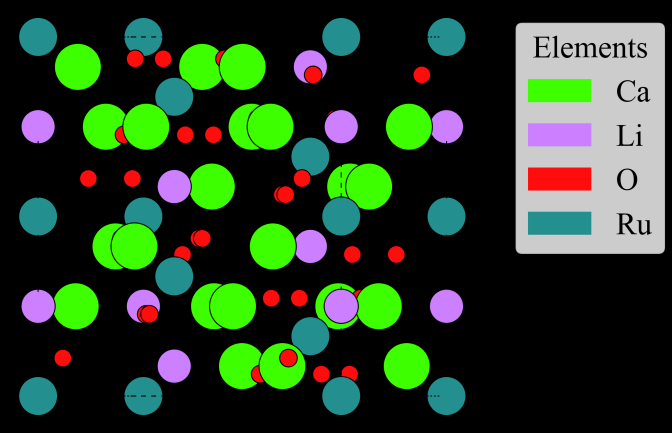
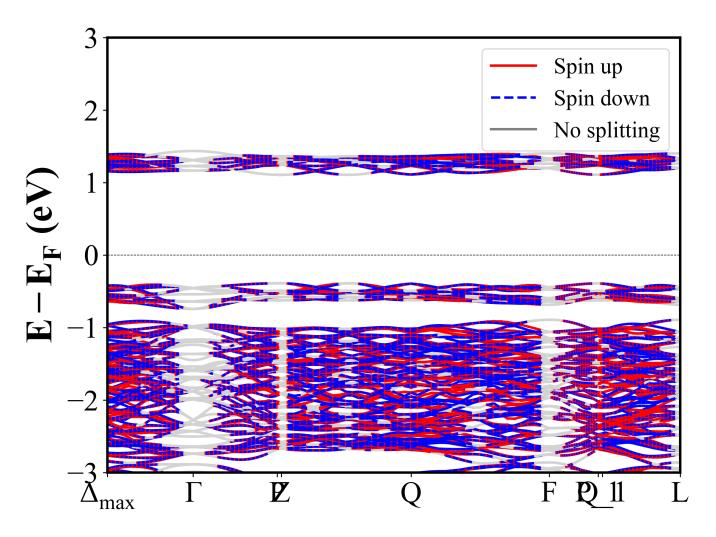
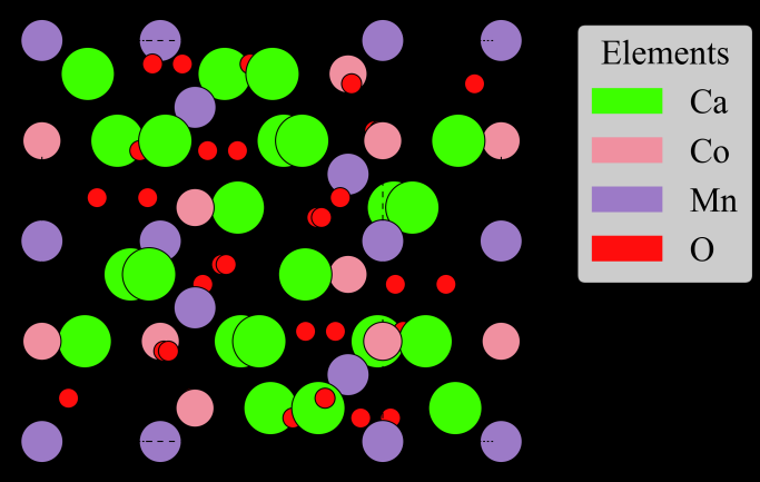
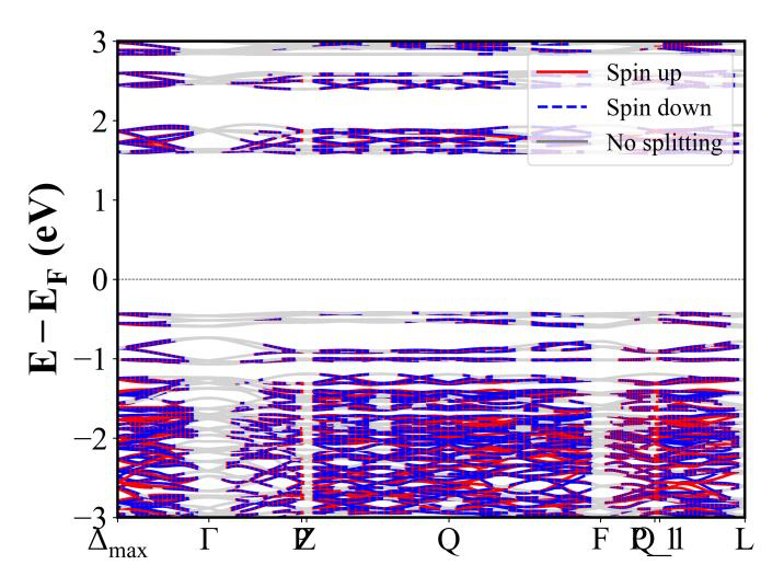
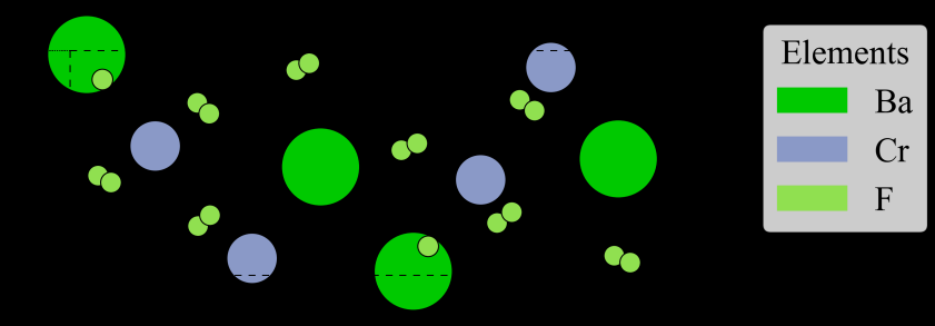
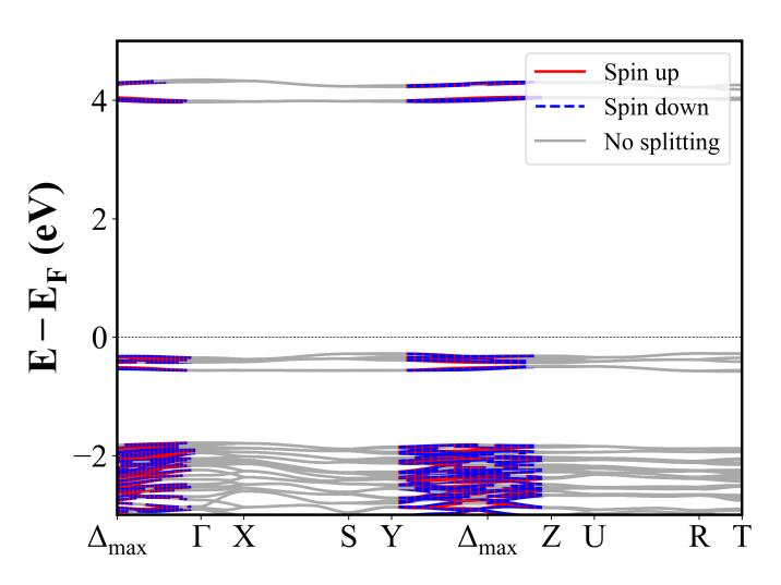
BaMn2V2O8 (I4_1cd) | Band Gap = 2.087 eV
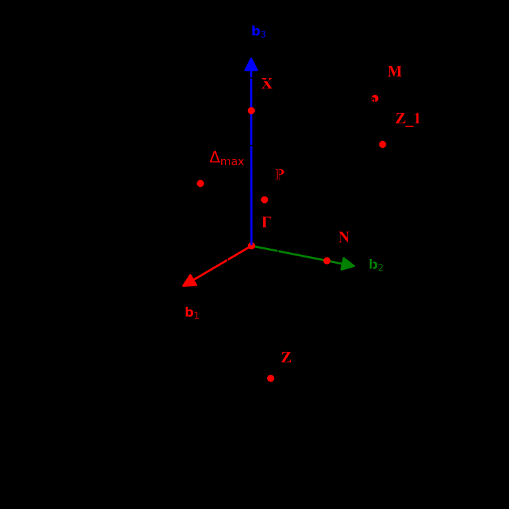
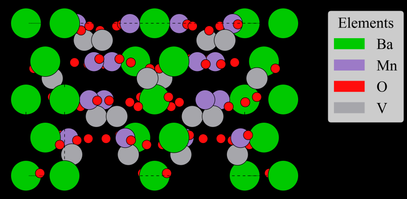
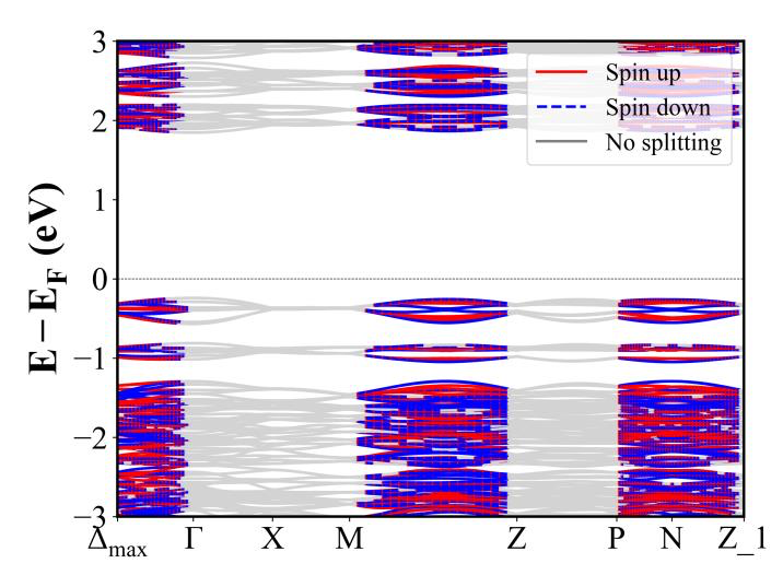
BaCuF4 (Cmc2_1) | Band Gap = 2.208 eV
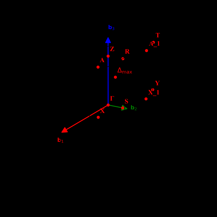
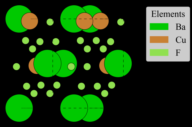
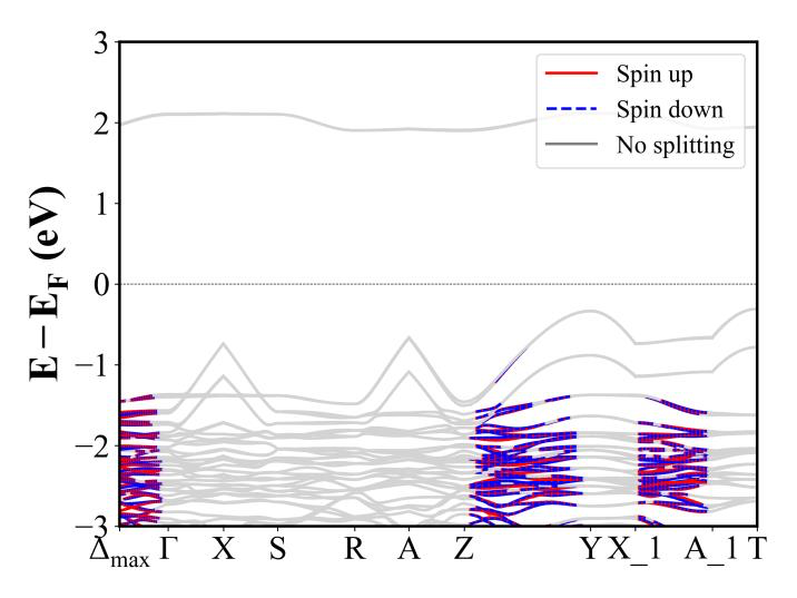
LiCa3OsO6 (R-3c) | Band Gap = 0.813 eV
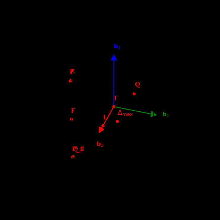
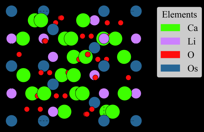
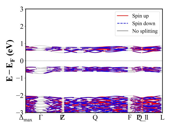
Ca(Al2Fe)4 (I4/mmm) | Band Gap = 0.000 eV
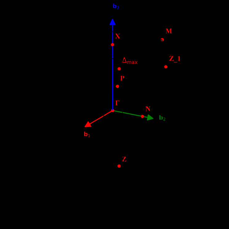
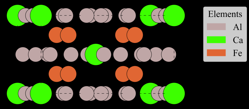
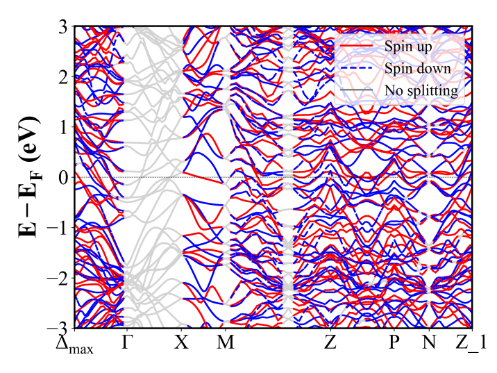
Ca2RuO4 (Pbca) | Band Gap = 0.664 eV
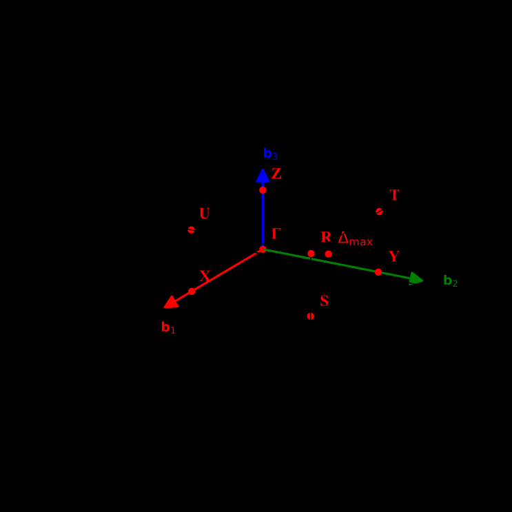
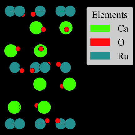
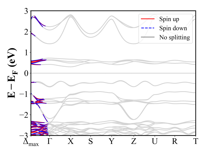
Ba2NdRuO6 (P2_1/c) | Band Gap = 1.026 eV
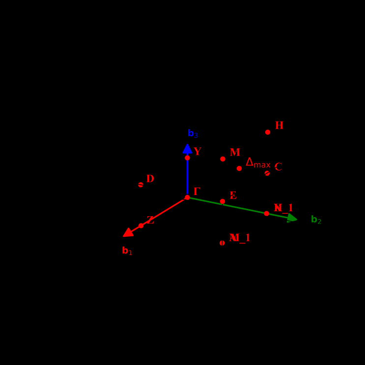
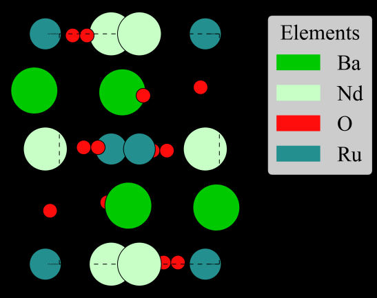
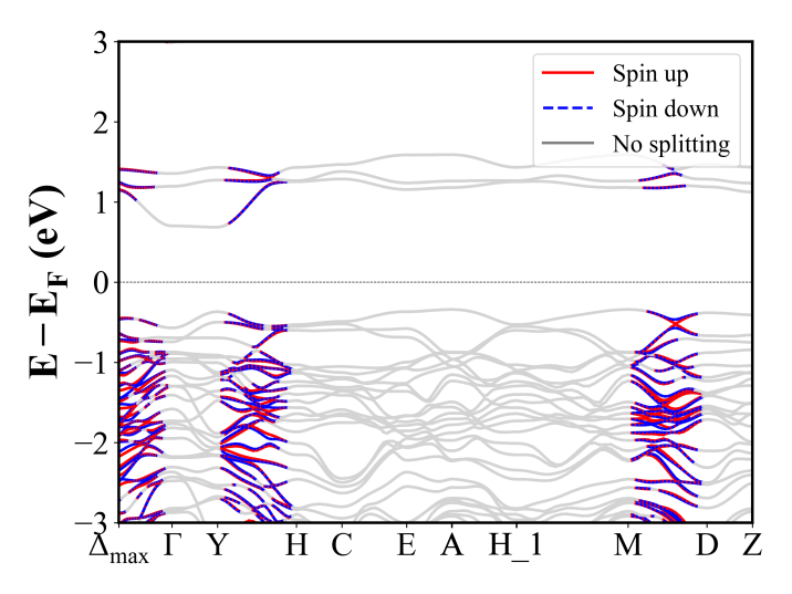
Ba3NiRu2O9 (P6_3/mmc) | Band Gap = 1.062 eV
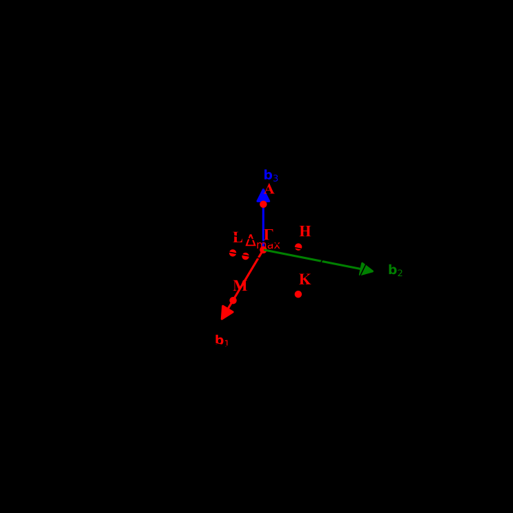
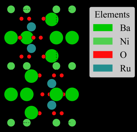
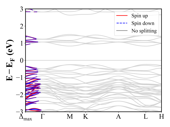
MnH6(CO2)3 (Pca2_1)
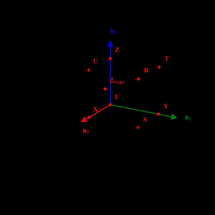
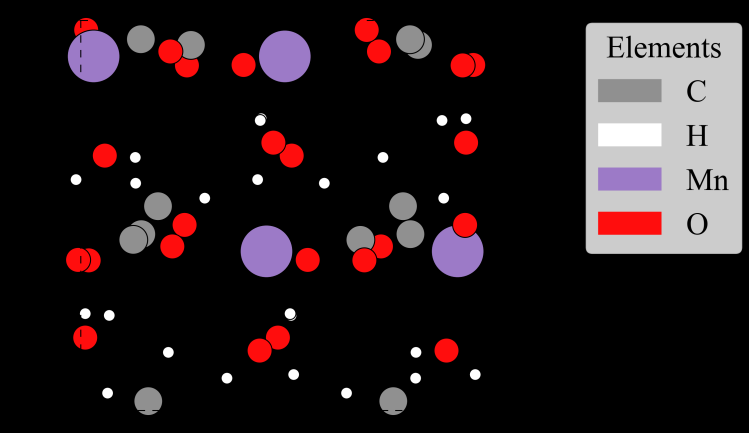
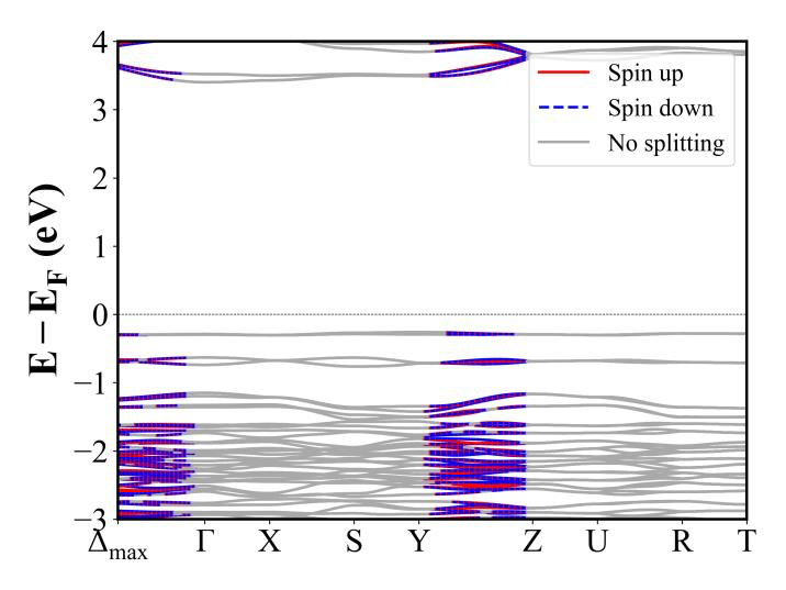
Ca2Fe2O5 (Pnma) | Band Gap = 1.373 eV
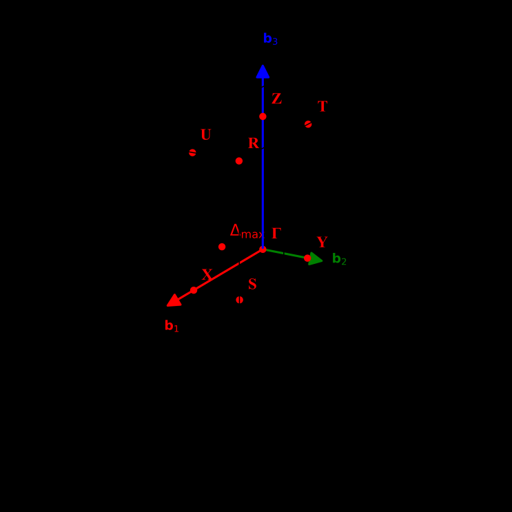
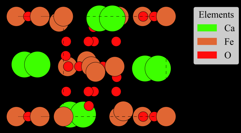
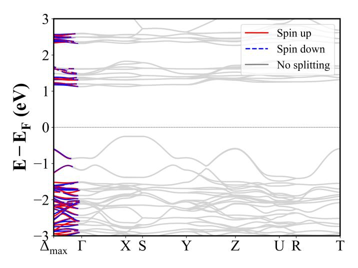
Ba2MnSi2O7 (P-42_1m) | Band Gap = 3.349 eV
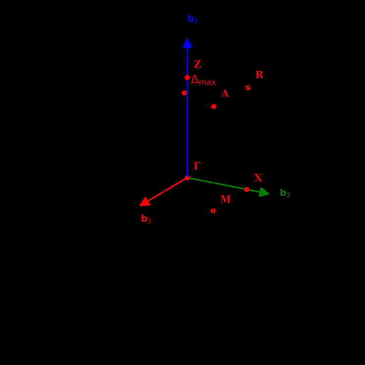
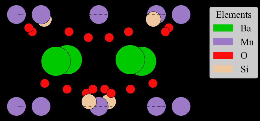
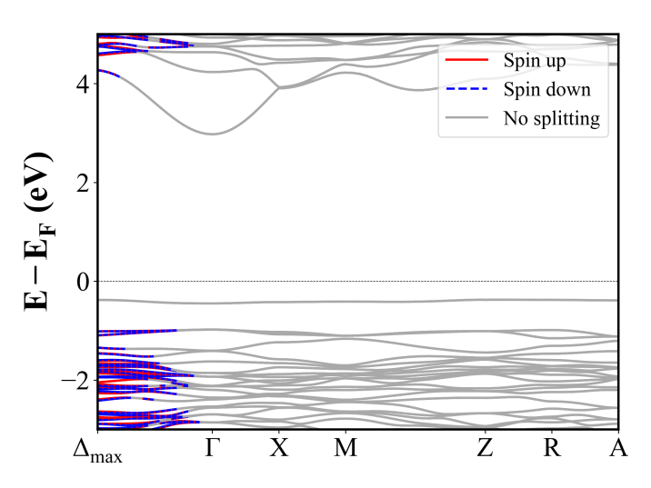
BaMnO3 (P6_3/mmc) | Band Gap = 2.613 eV
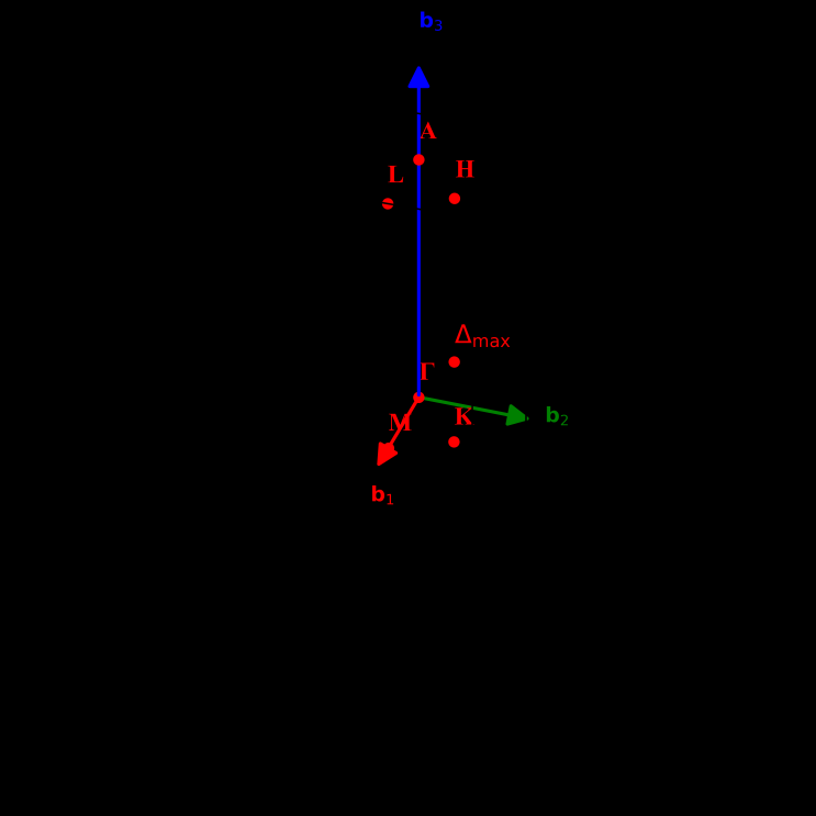
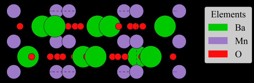
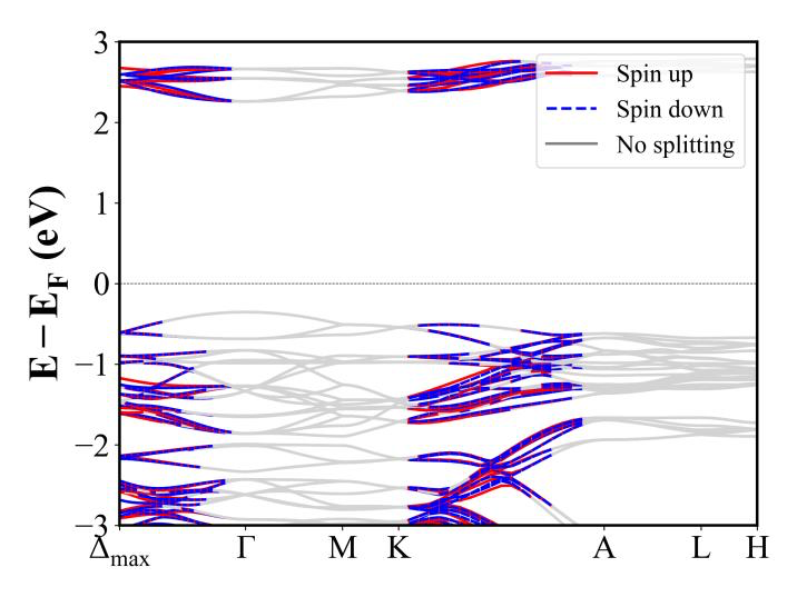
Ca2MnReO6 (P2_1/c) | Band Gap = 0.000 eV
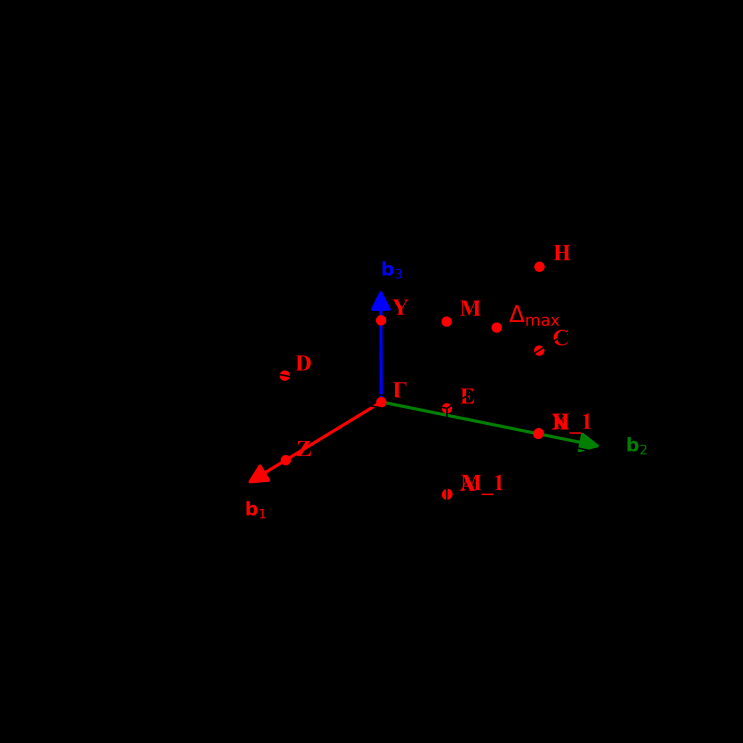
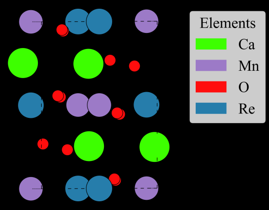
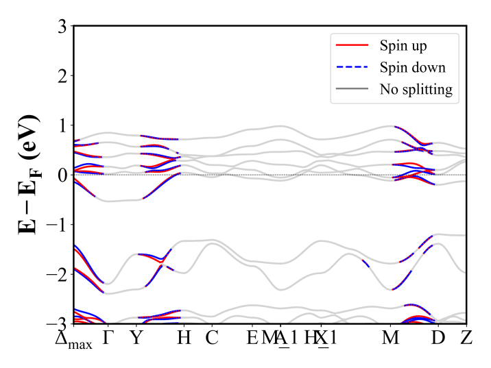
BaCoSiO4 (P6_3) | Band Gap = 3.079 eV
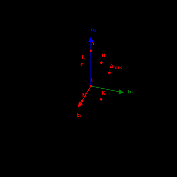
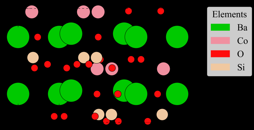
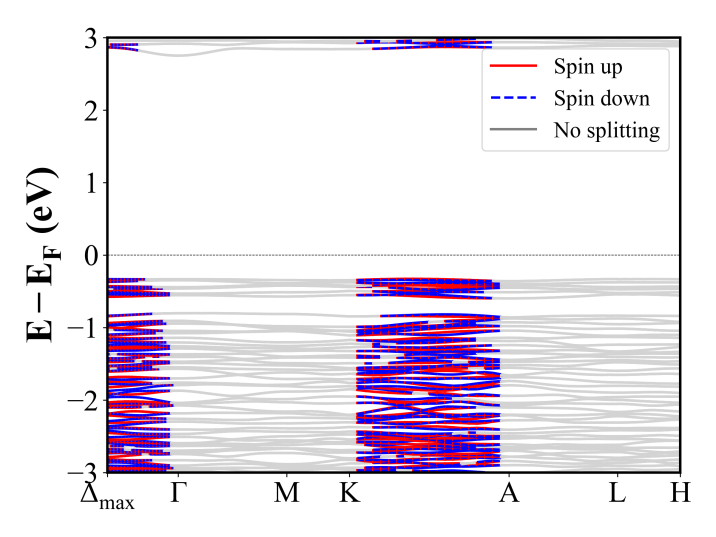
Ba3MnSb2O9 (C2/c) | Band Gap = 2.075 eV
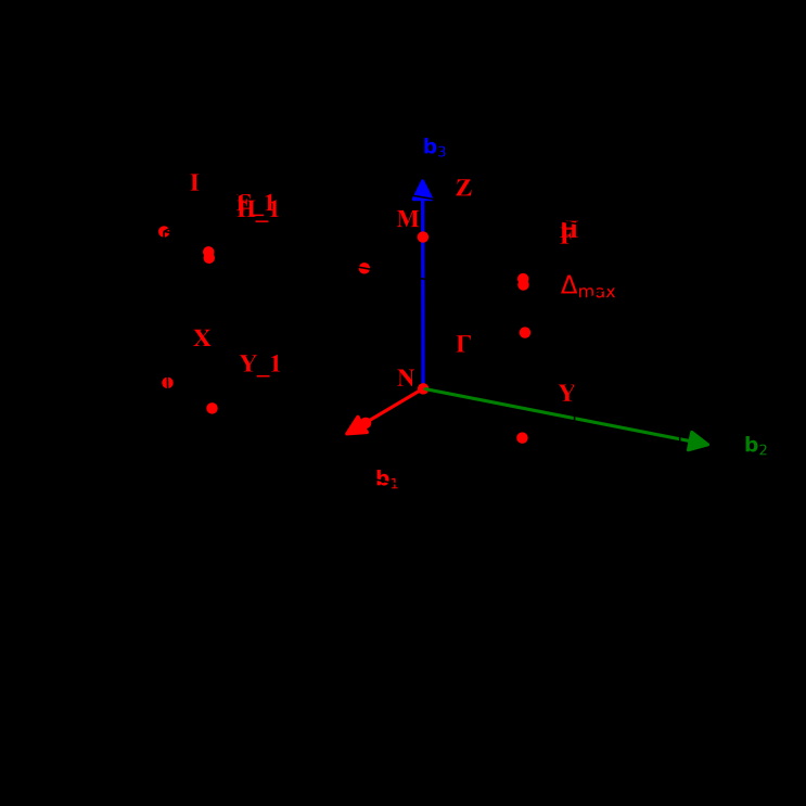
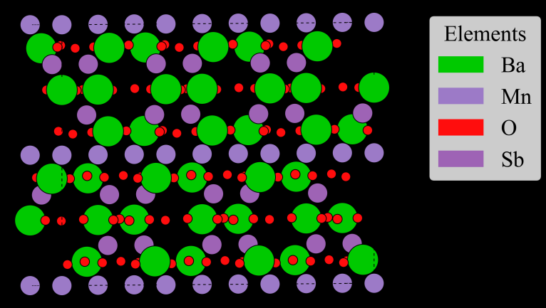
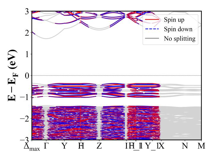
Ba2CoGe2O7 (P-42_1m) | Band Gap = 2.592 eV
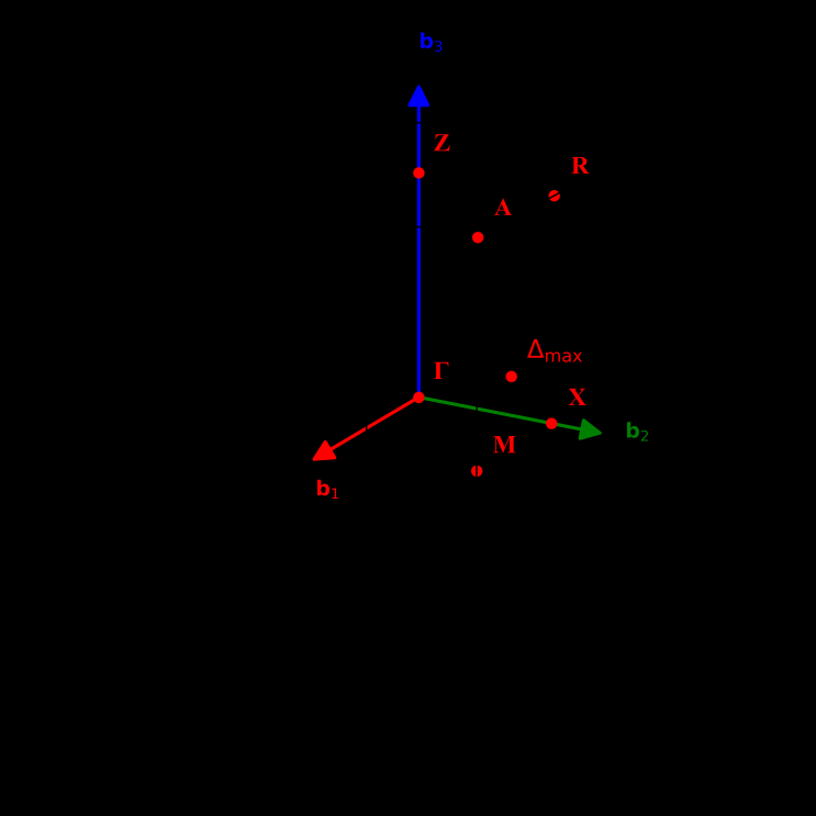
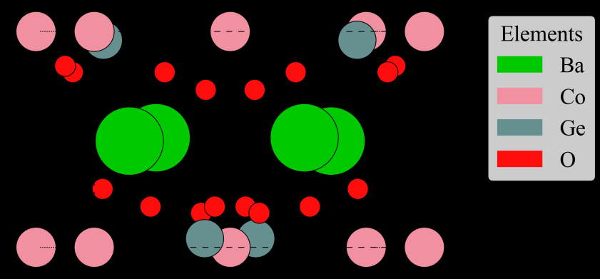
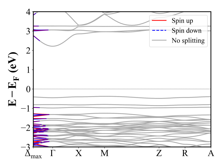
CoH9C4NO6 (Pnma) | Band Gap = 3.236 eV
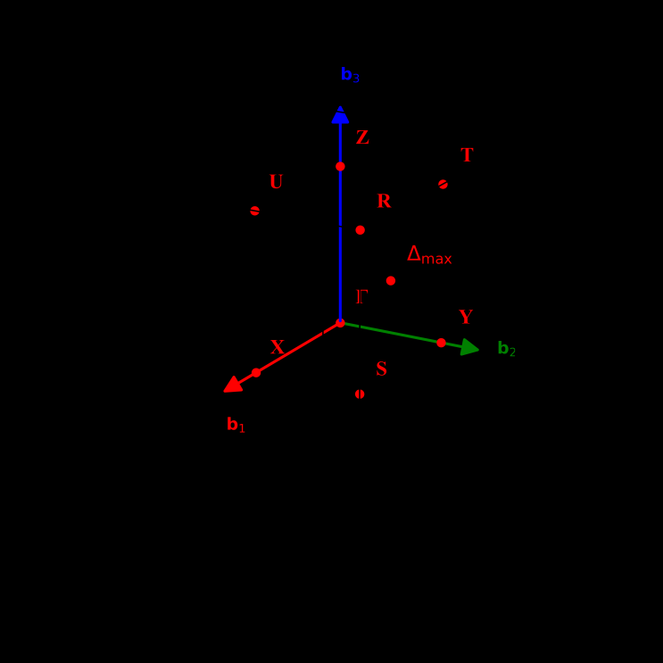
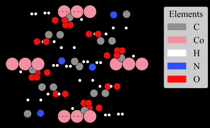
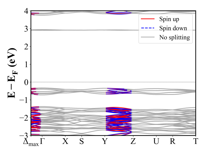
VCrO4 (Cmcm) | Band Gap = 2.877 eV
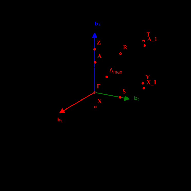
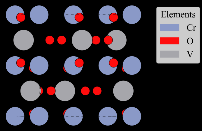
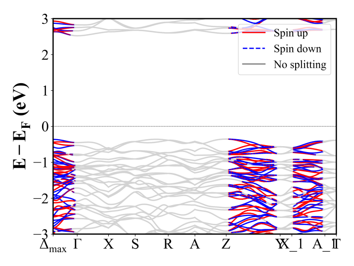
CoF2 (P4_2/mnm) | Band Gap = 3.306 eV
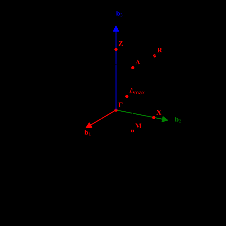
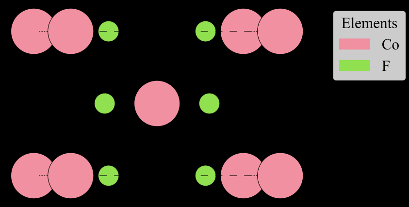
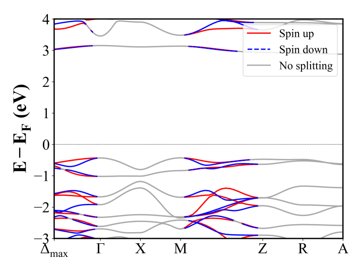
CaNi3(P2O7)2 (P2_1/c) | Band Gap = 4.464 eV
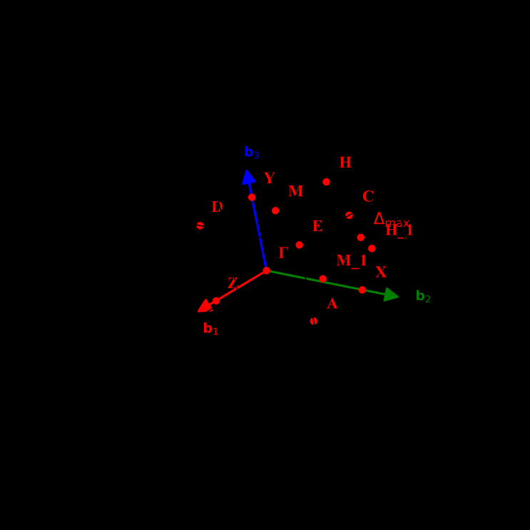
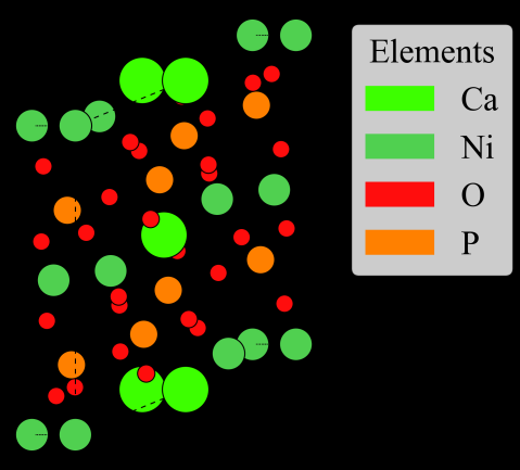
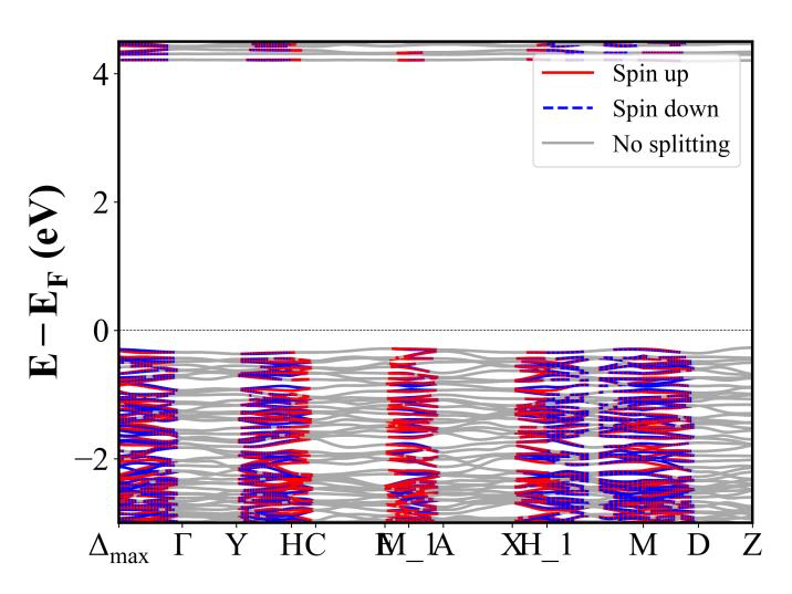
CaIrO3 (Cmcm) | Band Gap = 0.038 eV
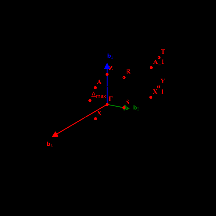
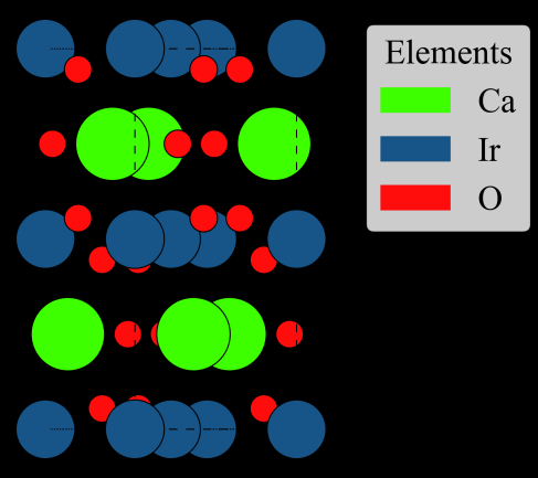
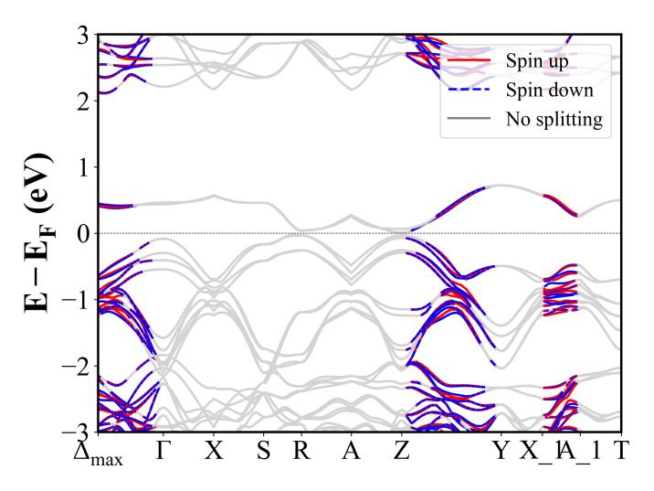
CoF3 (R-3c) | Band Gap = 1.825 eV
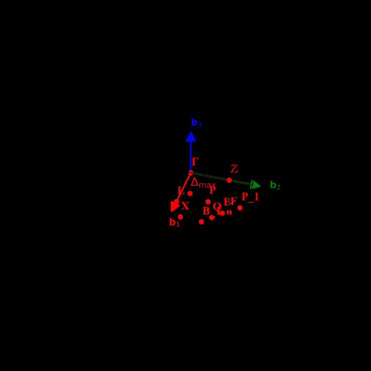
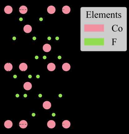
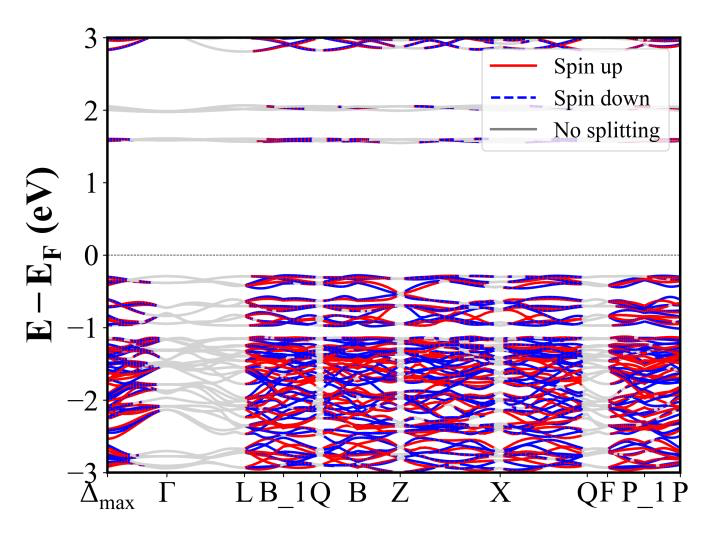
Nb4CrS8 (P6_3/mmc) | Band Gap = 0.000 eV
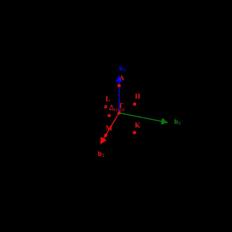
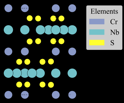
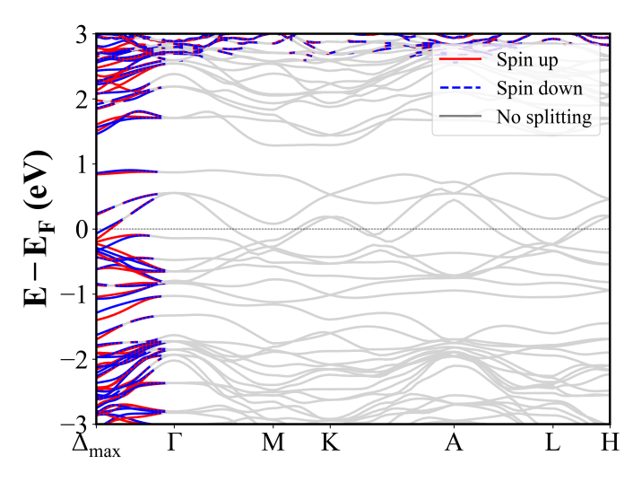
CeFeO3 (Pnma) | Band Gap = 2.825 eV
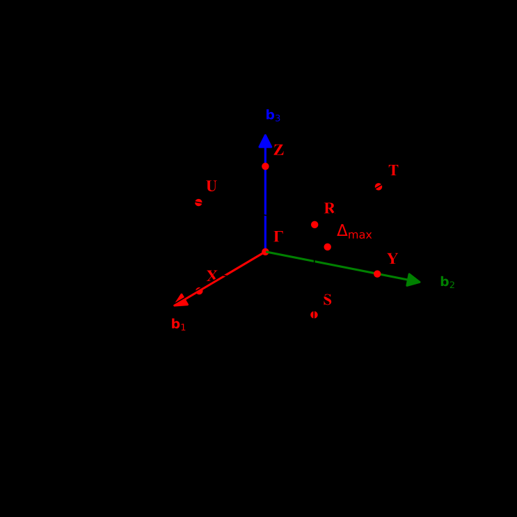
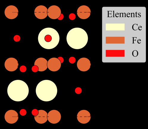
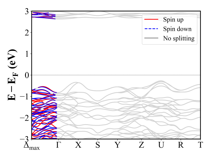
Co2Mo3O8 (P6_3mc) | Band Gap = 0.000 eV
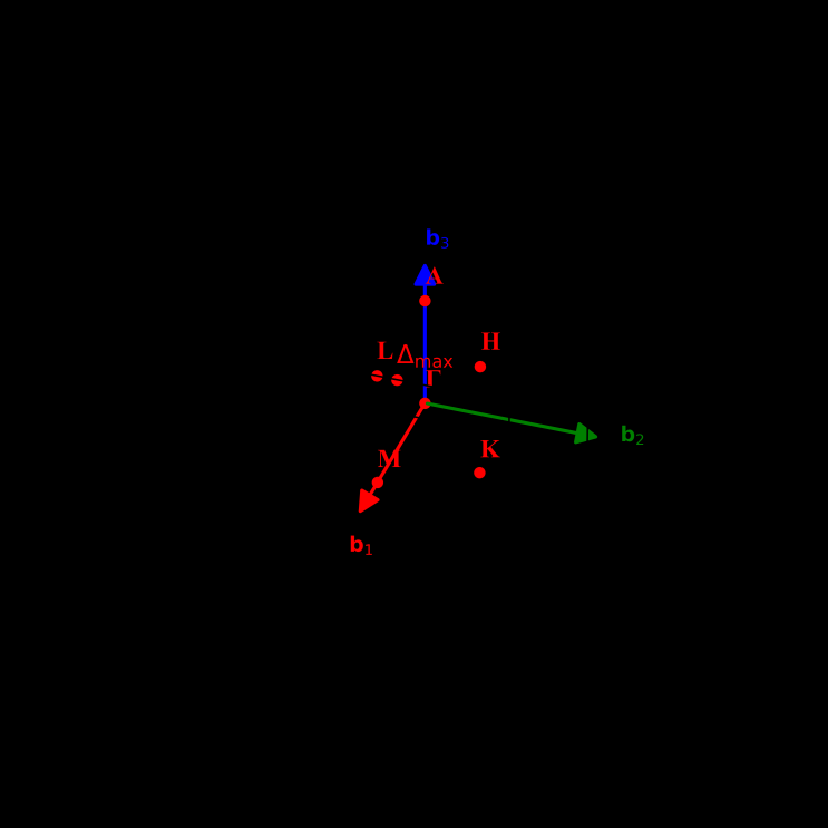
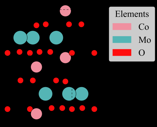
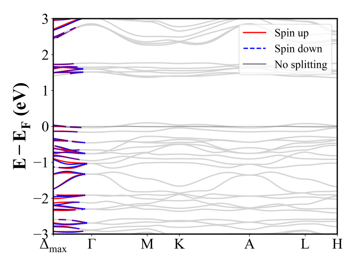
FeCoPO5 (Pnma) | Band Gap = 2.399 eV
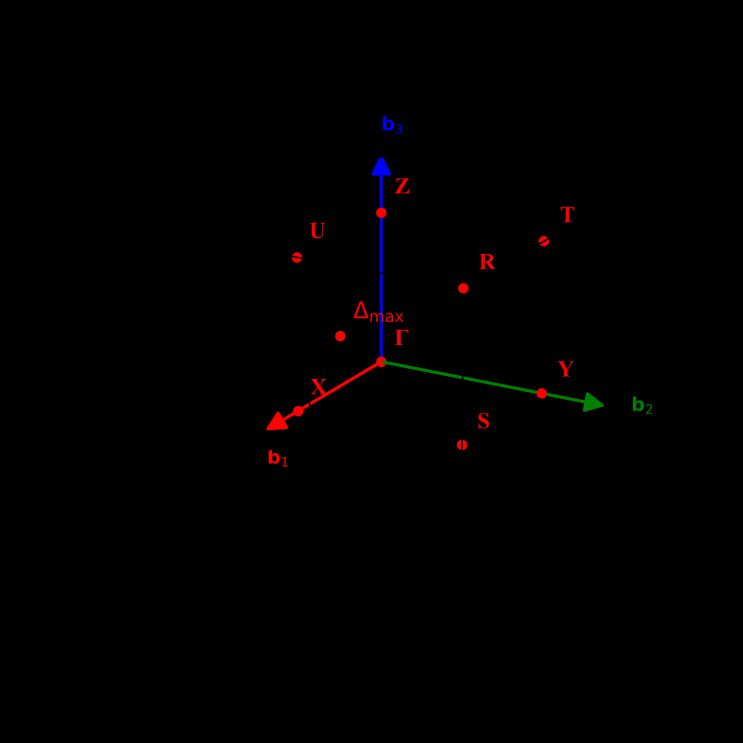
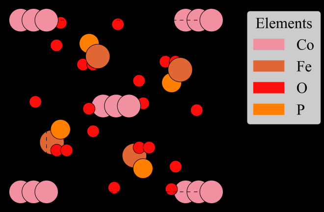
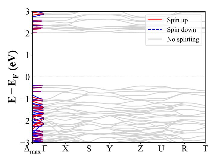
CsCoCl3 (P6_3/mmc) | Band Gap = 2.546 eV
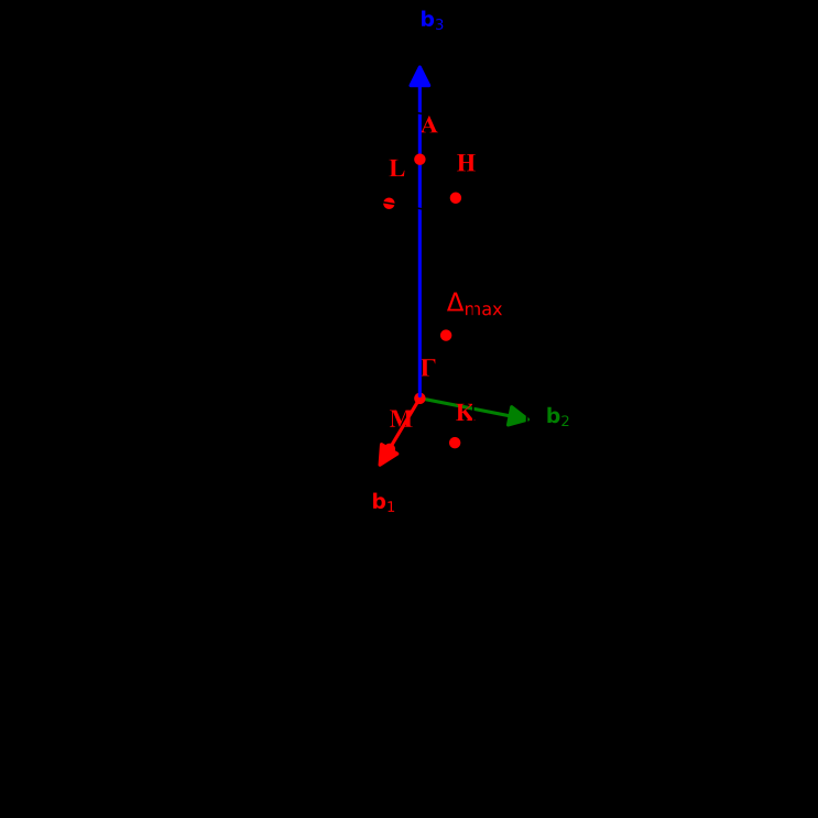
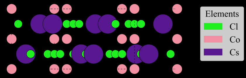
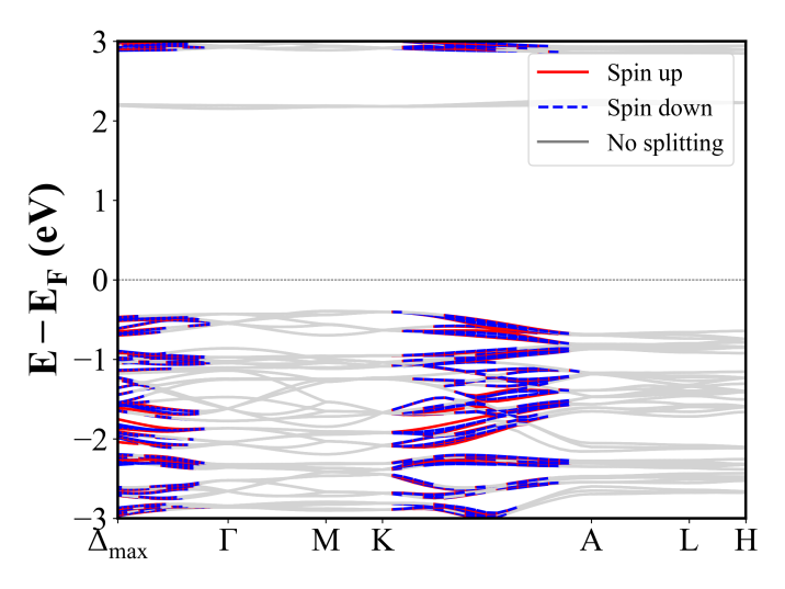
Ta4CoSe8 (P6_3/mmc) | Band Gap = 0.000 eV
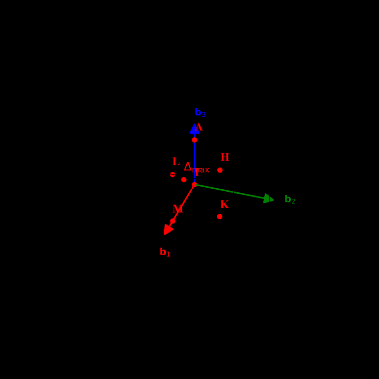
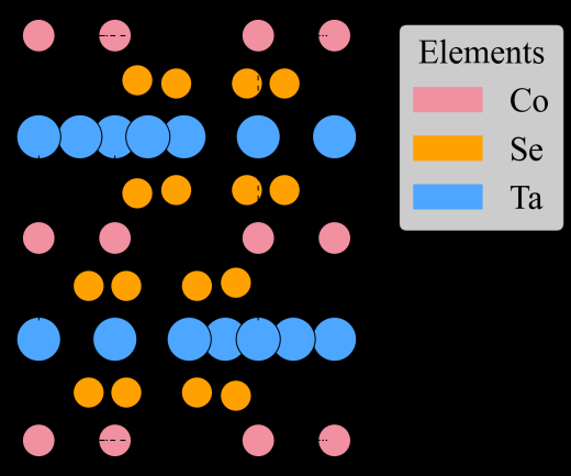
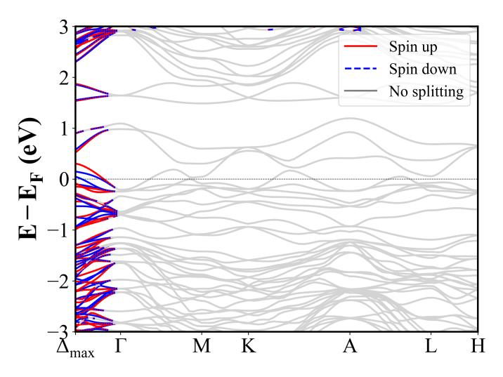
CoCO3 (R-3c) | Band Gap = 2.766 eV
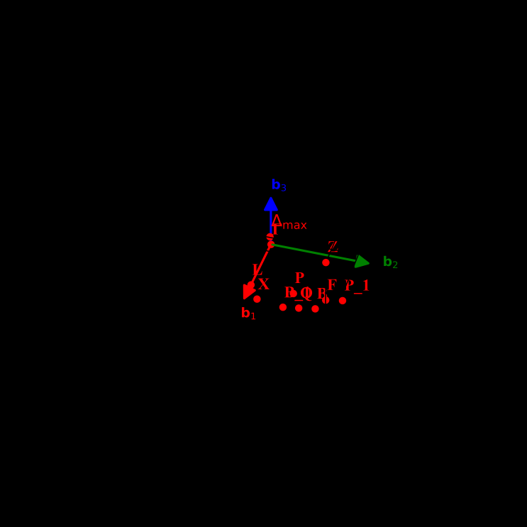
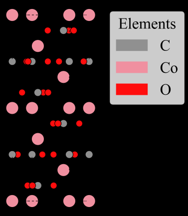
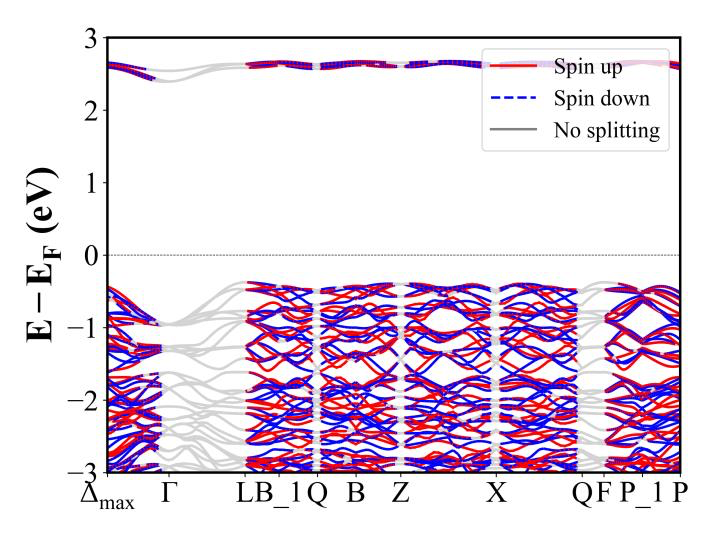
CrSb (P6_3/mmc) | Band Gap = 0.000 eV
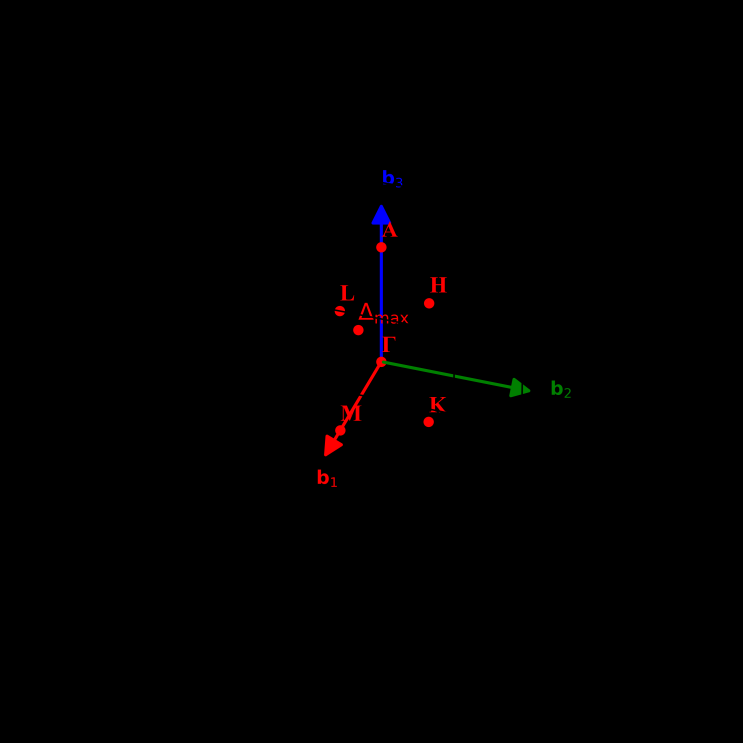
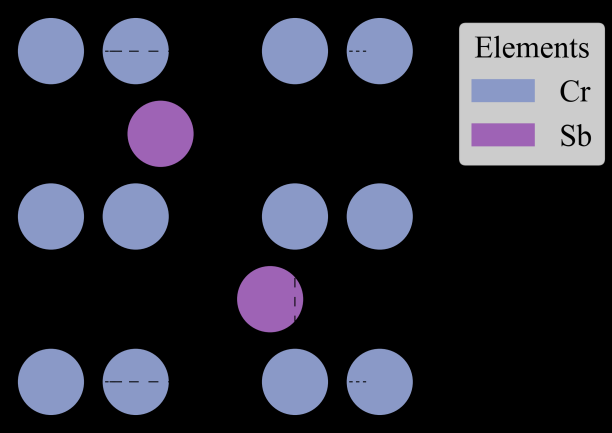
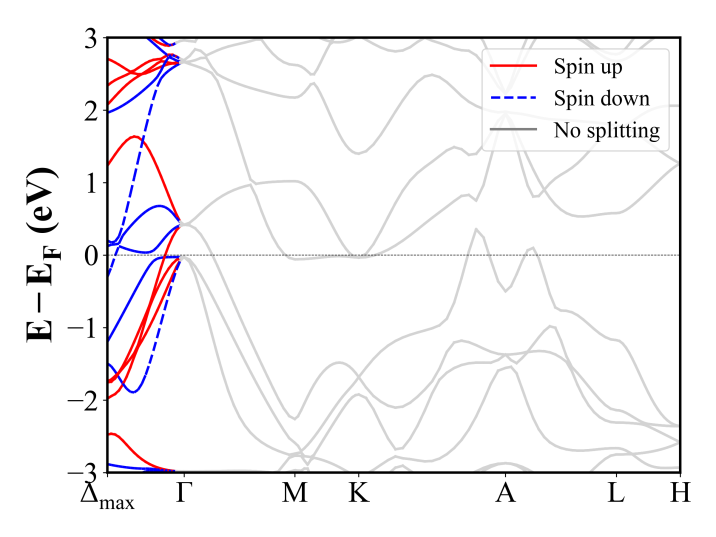
CeMn2(GeO3)4 (P4/nbm) | Band Gap = 0.000 eV
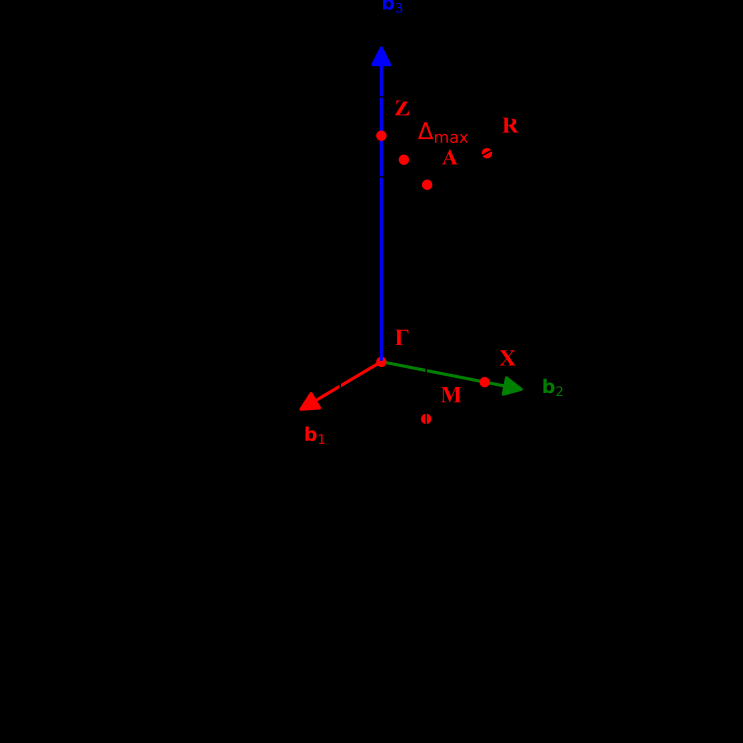
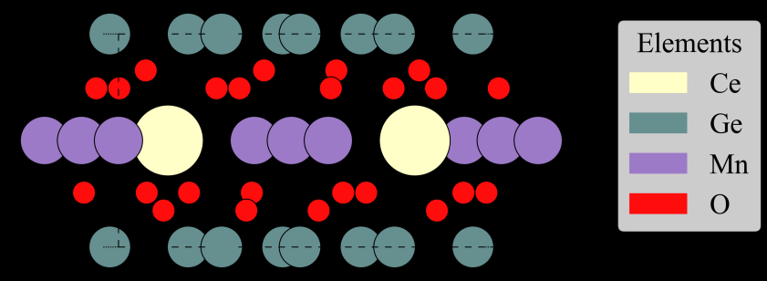
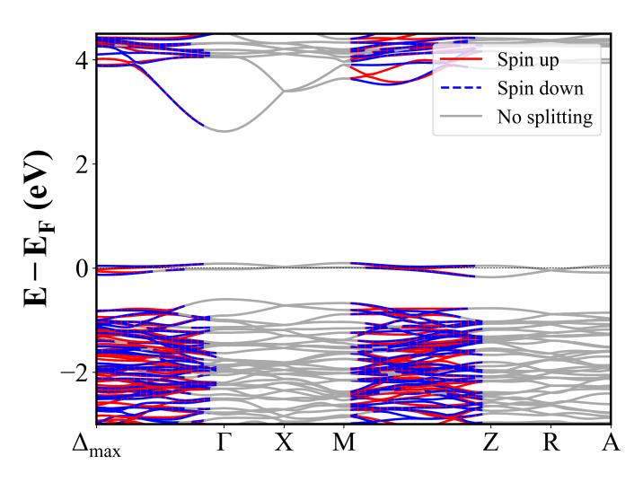
Ce4Sb3 (I-43d) | Band Gap = 0.000 eV
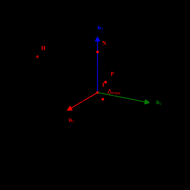
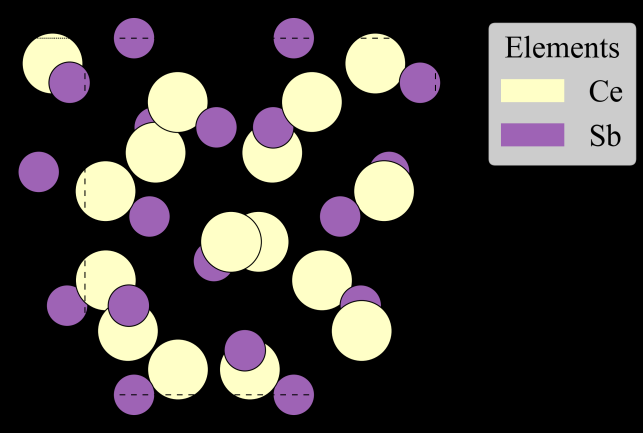
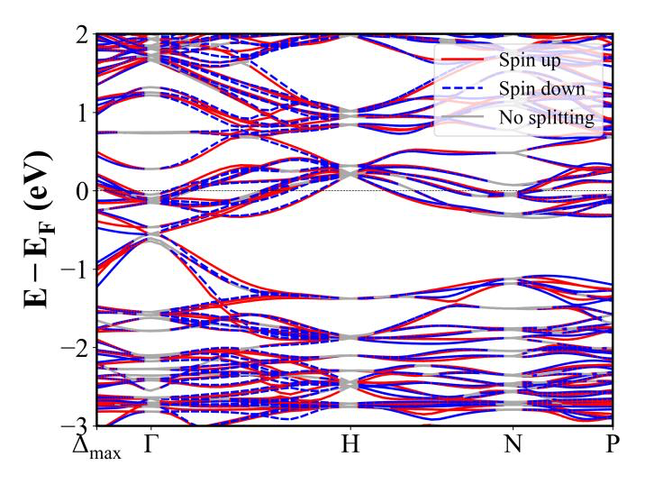
CsCoF4 (I-4c2) | Band Gap = 2.099 eV
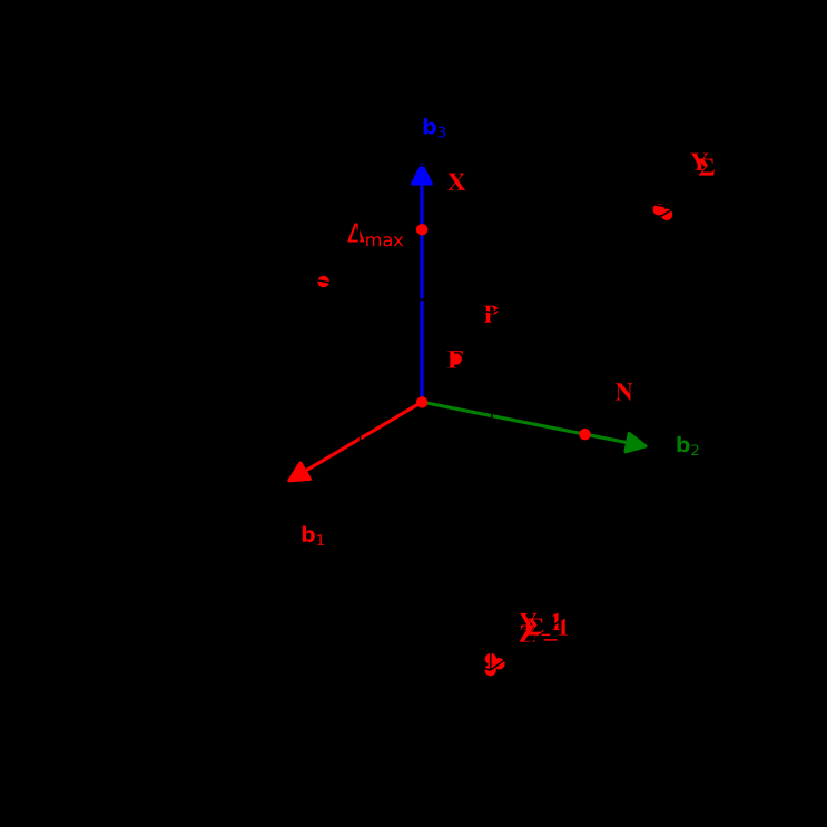
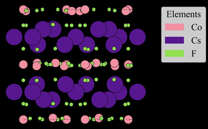
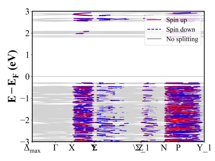
Co2SiO4 (Pnma) | Band Gap = 2.505 eV
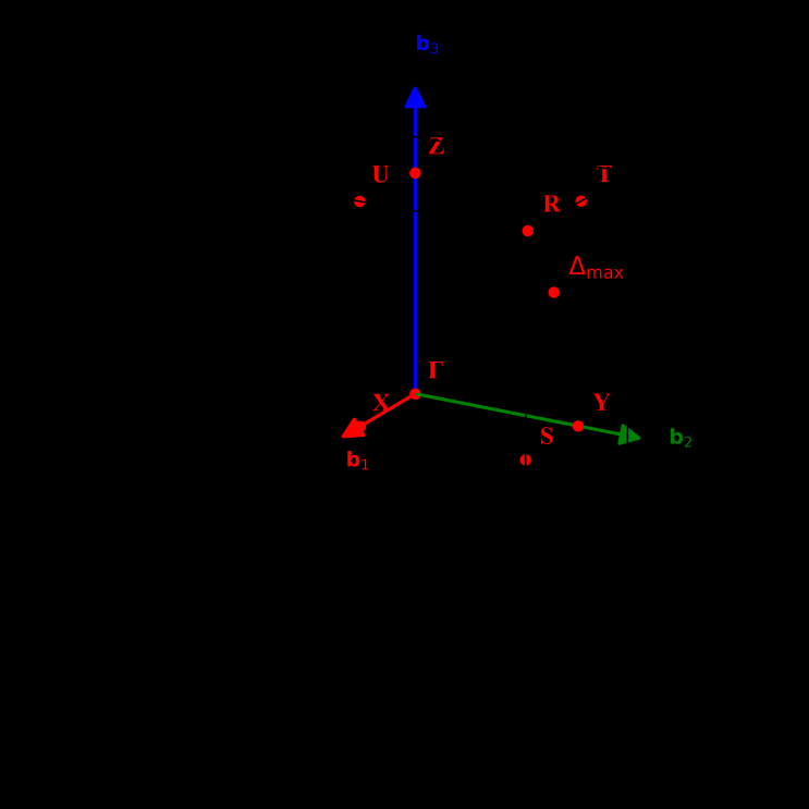
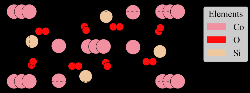
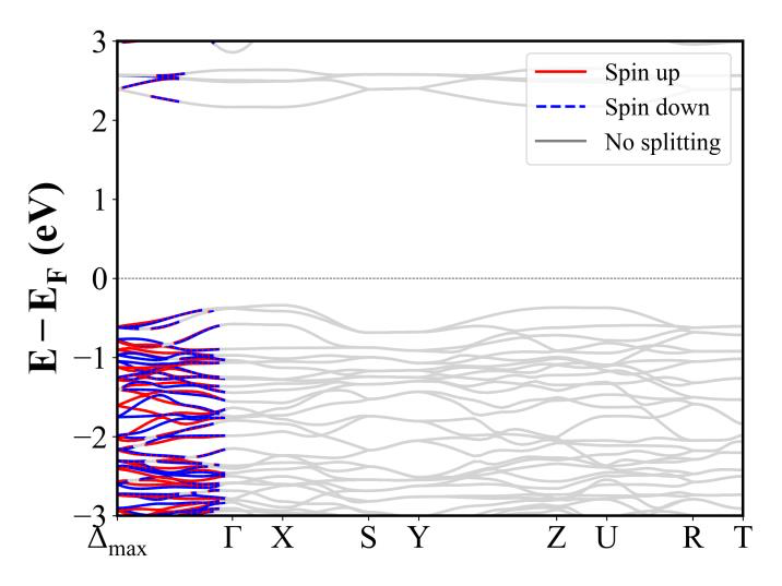
CsMn2F6 (Pnma) | Band Gap = 1.529 eV
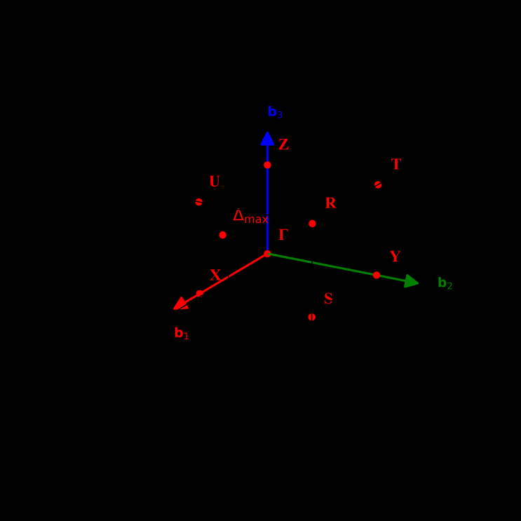
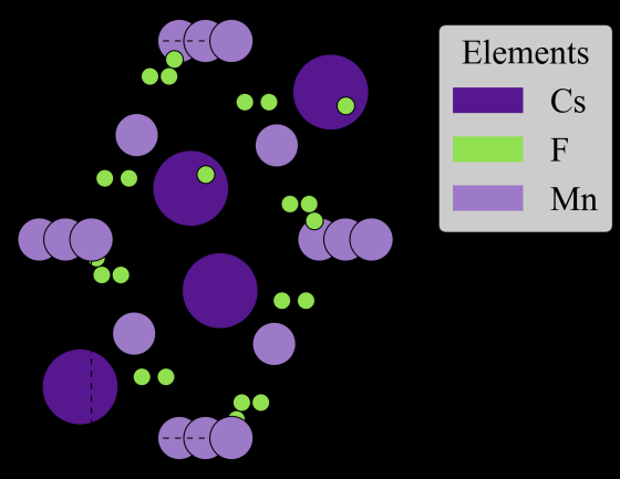
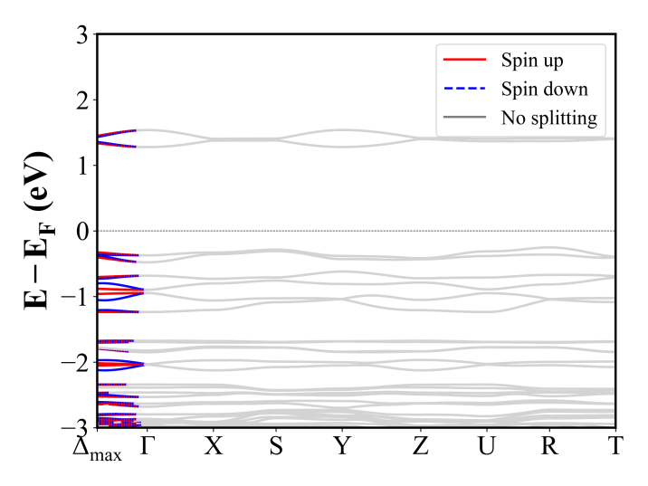
CoH6(CO3)2 (P2_1/c) | Band Gap = 1.908 eV
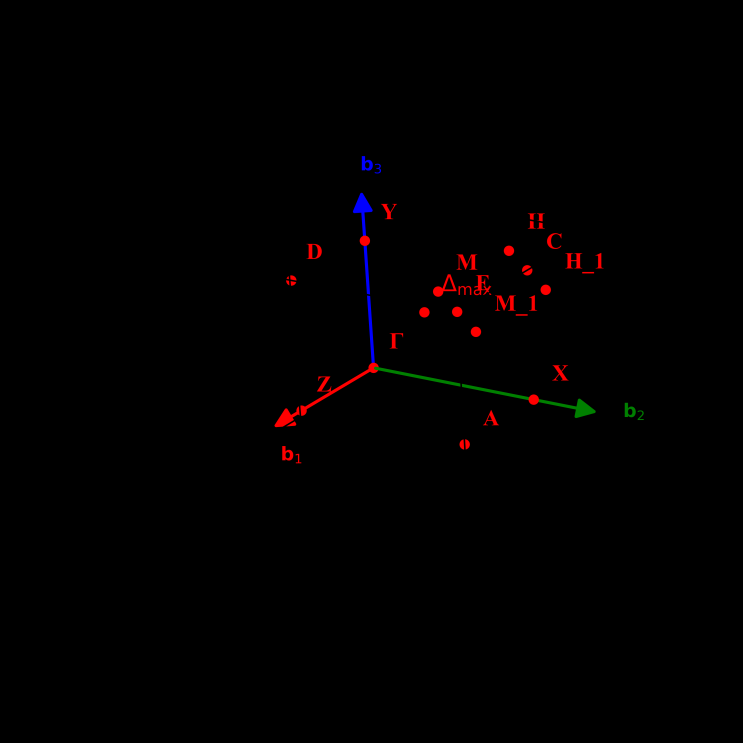
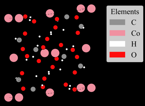
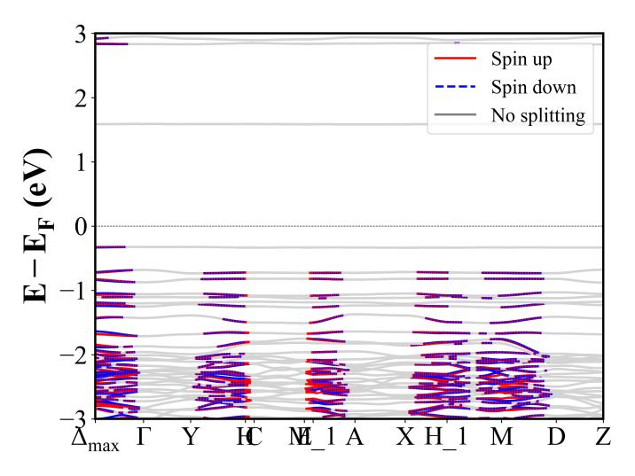
CrSe (P6_3/mmc) | Band Gap = 0.000 eV
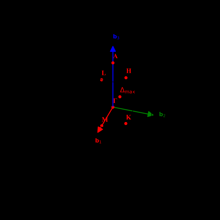
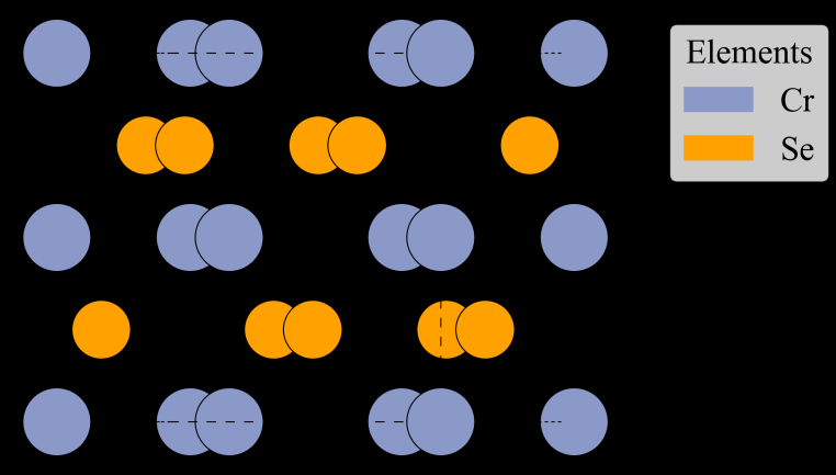
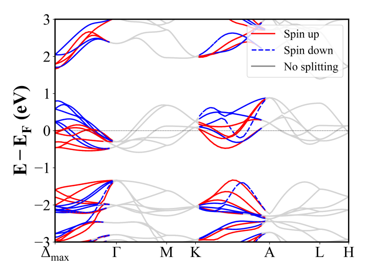
FeCuPO5 (Pnma) | Band Gap = 1.955 eV
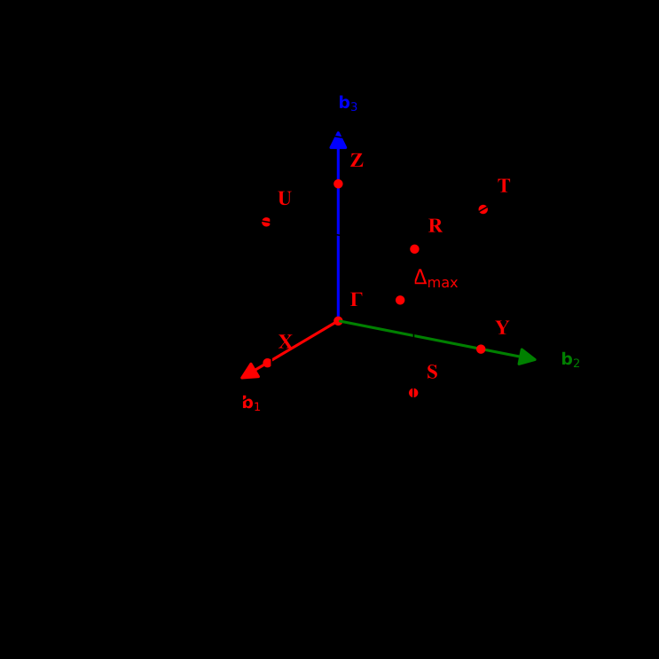
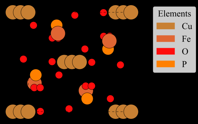
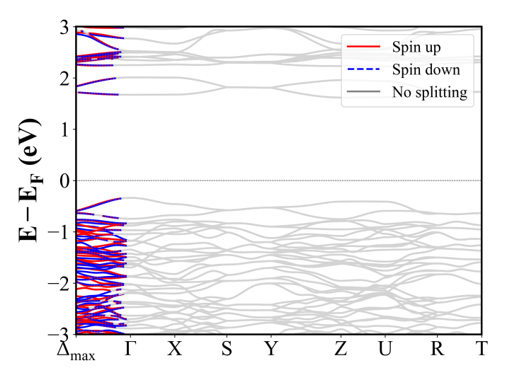
Cu2H3ClO3 (P2_1/c) | Band Gap = 1.749 eV
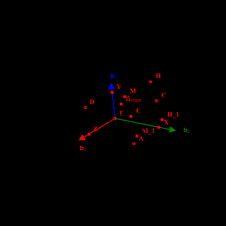
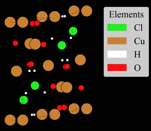
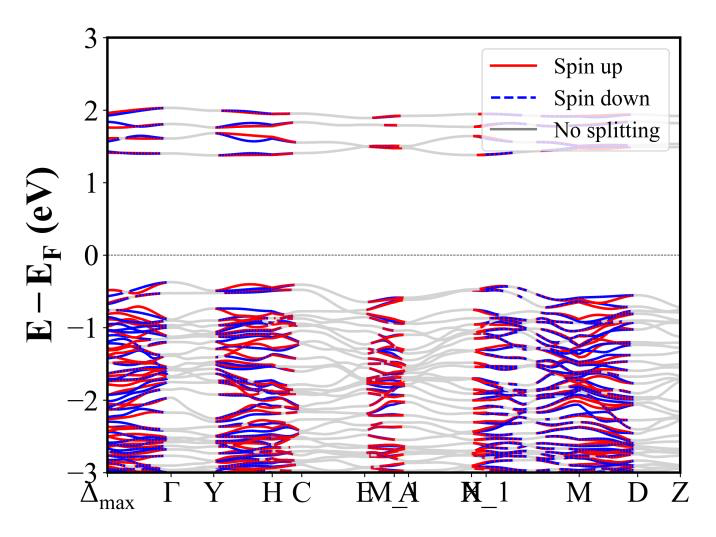
Cu3Mo2O9 (Pnma) | Band Gap = 1.236 eV
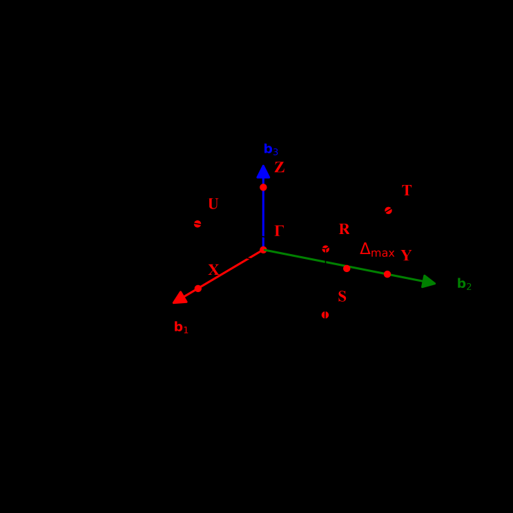
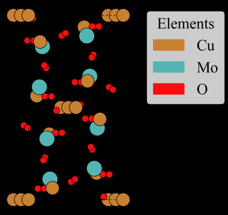
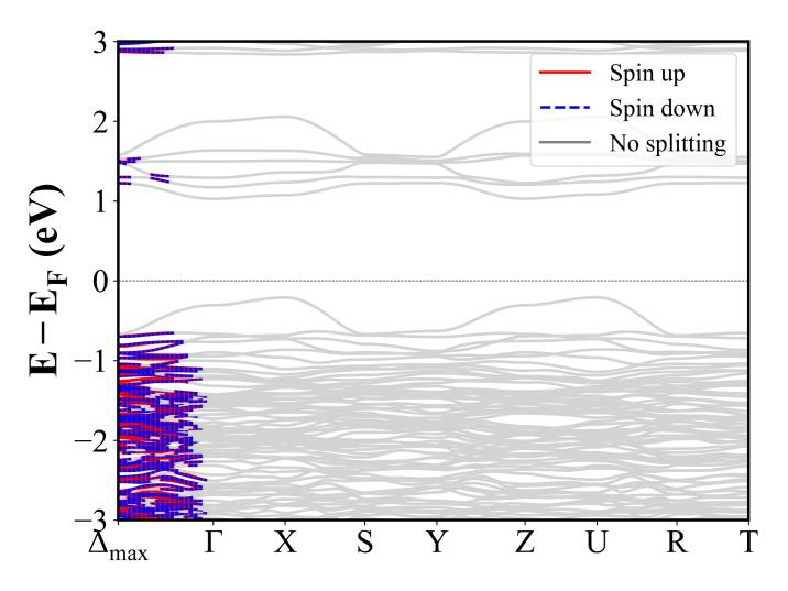
DyCrO3 (Pnma) | Band Gap = 3.079 eV
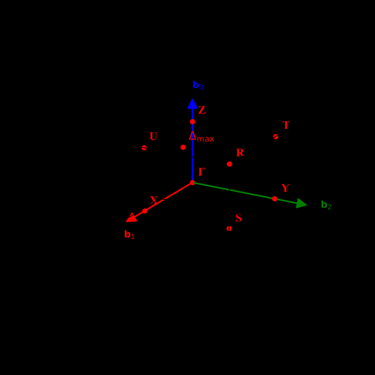
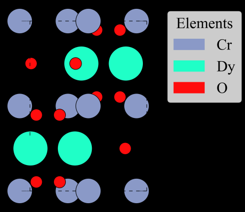
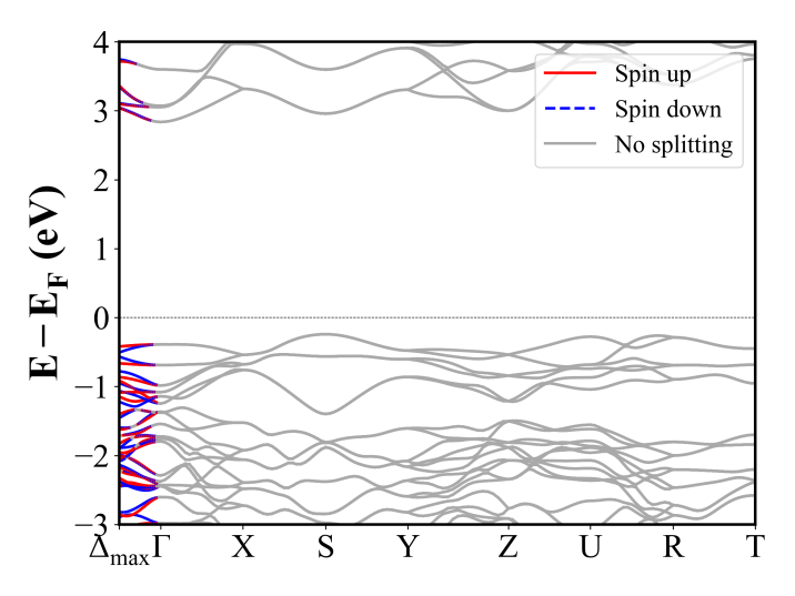
Cu4H6BrO6F (Pnma) | Band Gap = 1.714 eV
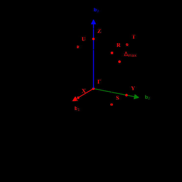
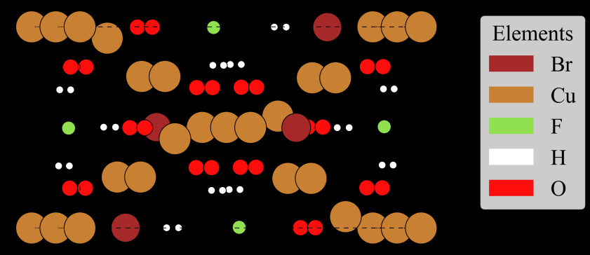
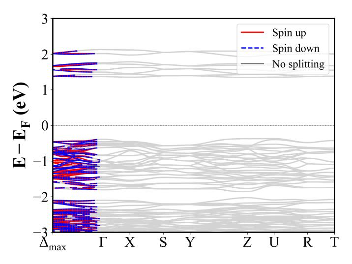
CsMnBr3 (P6_3/mmc) | Band Gap = 3.828 eV
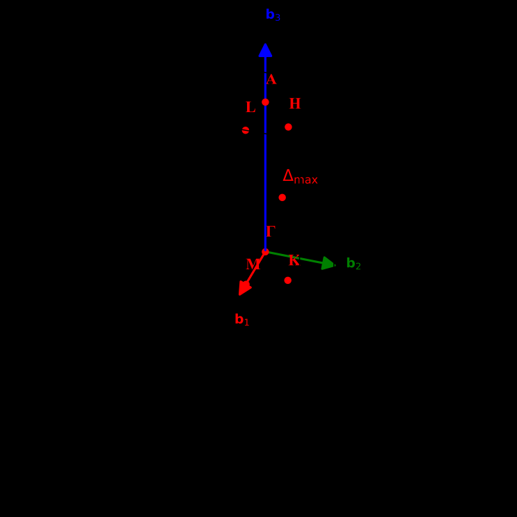
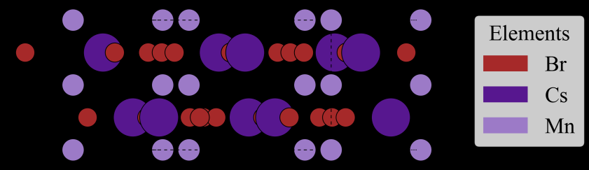
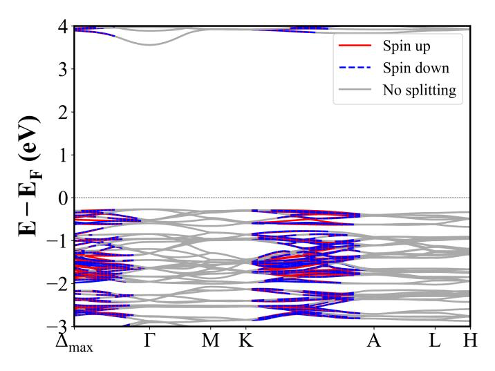
FeCuS2 (I-42d) | Band Gap = 1.043 eV
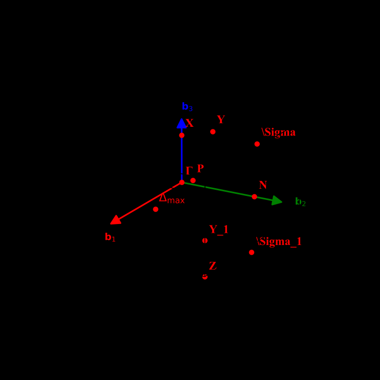
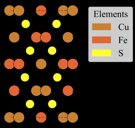
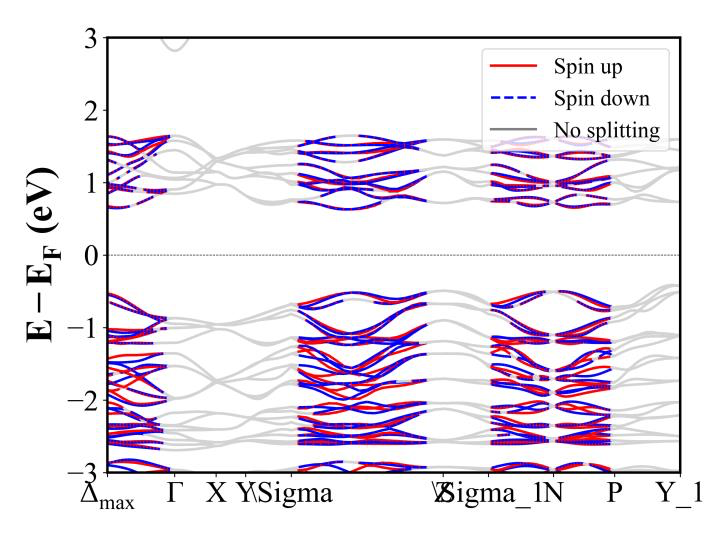
Cu2ClO3 (P2_1/c) | Band Gap = 0.000 eV
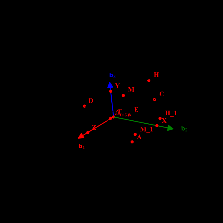
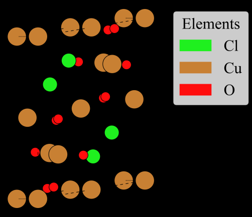
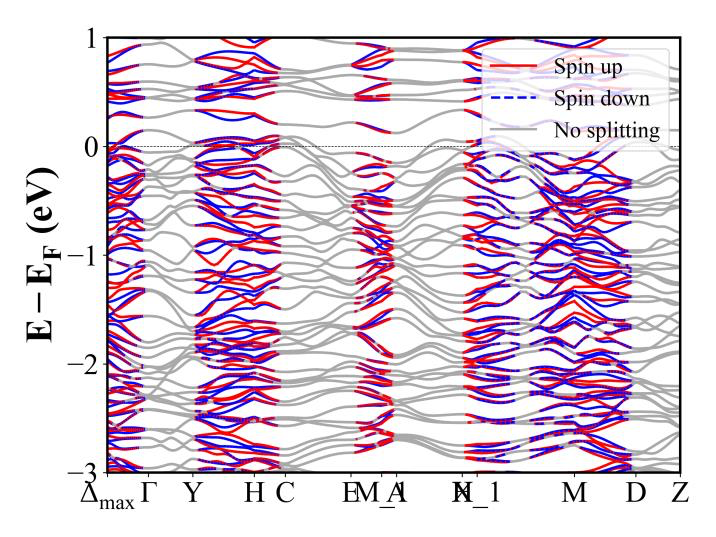
Er2Cu2O5 (Pna2_1) | Band Gap = 1.732 eV
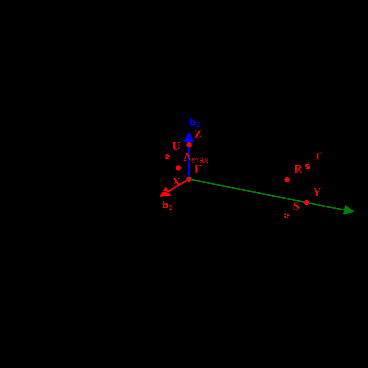
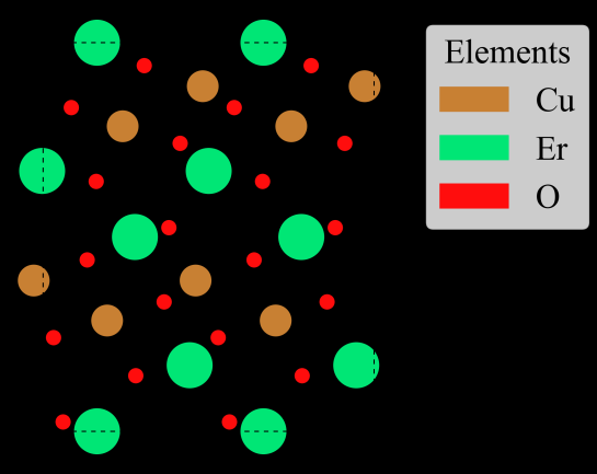
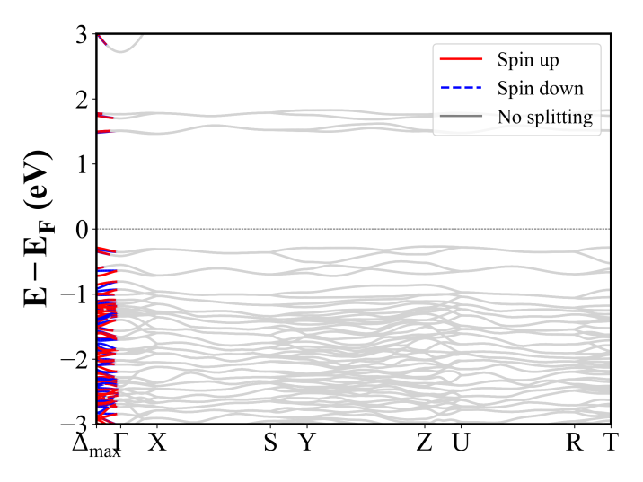
Cu(BO2)2 (I-42d) | Band Gap = 2.137 eV
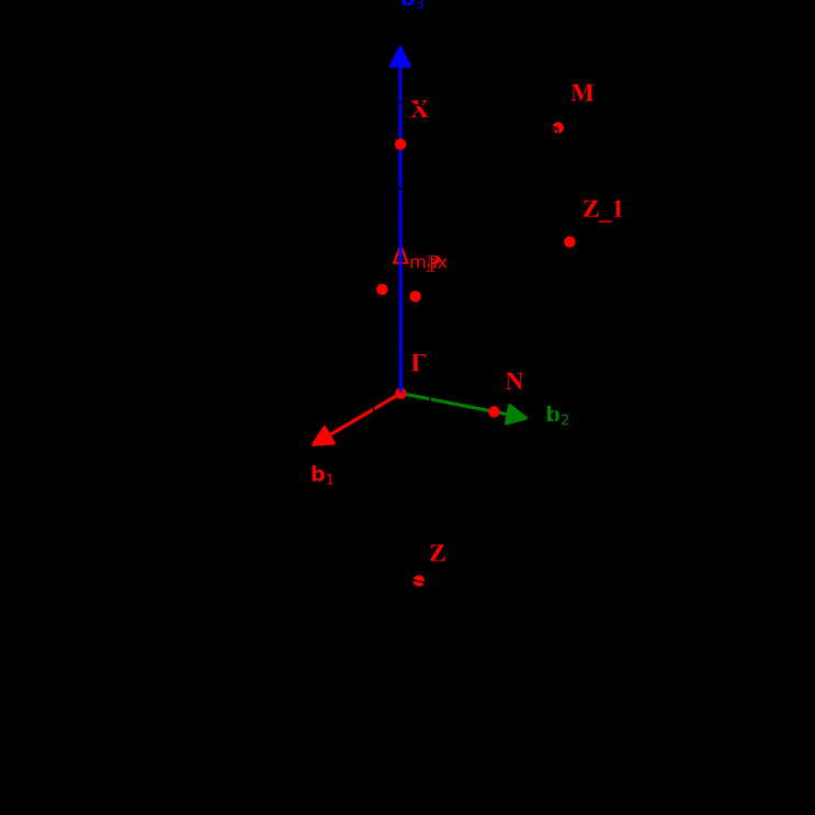
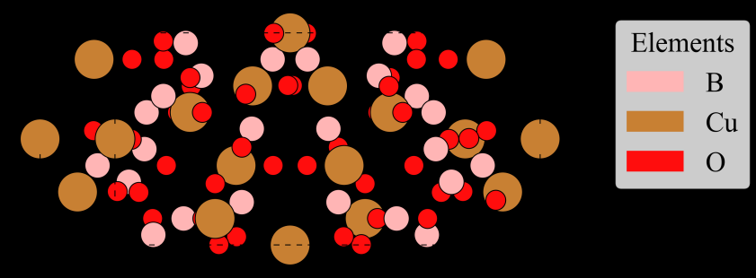
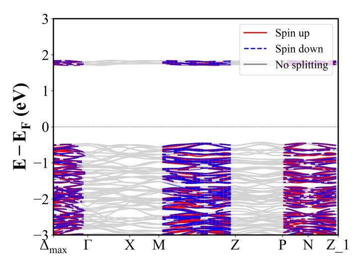
CsNiC3(SN)3 (P2_1/c) | Band Gap = 2.843 eV
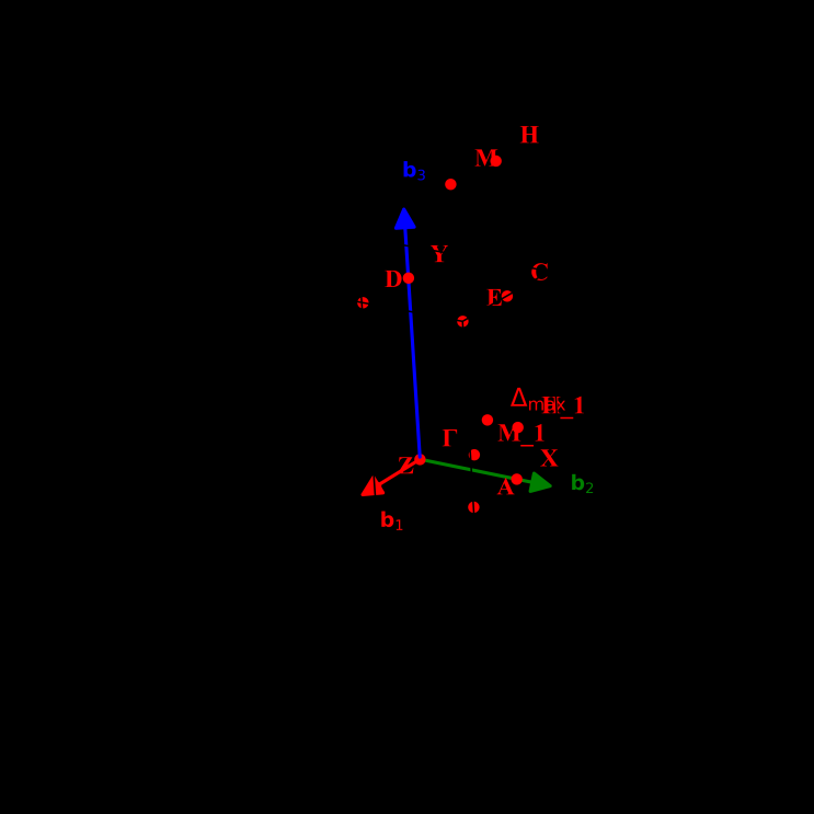
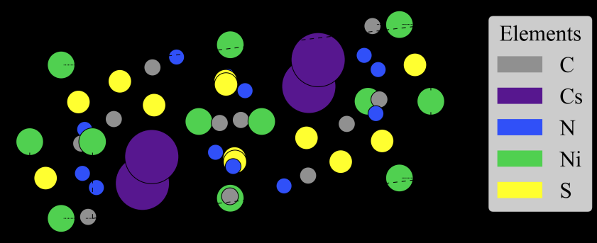
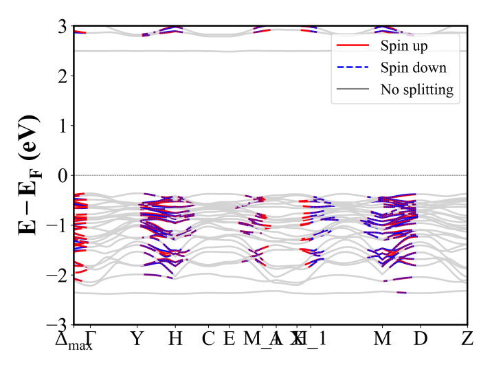
DyCrWO6 (Pna2_1) | Band Gap = 1.912 eV
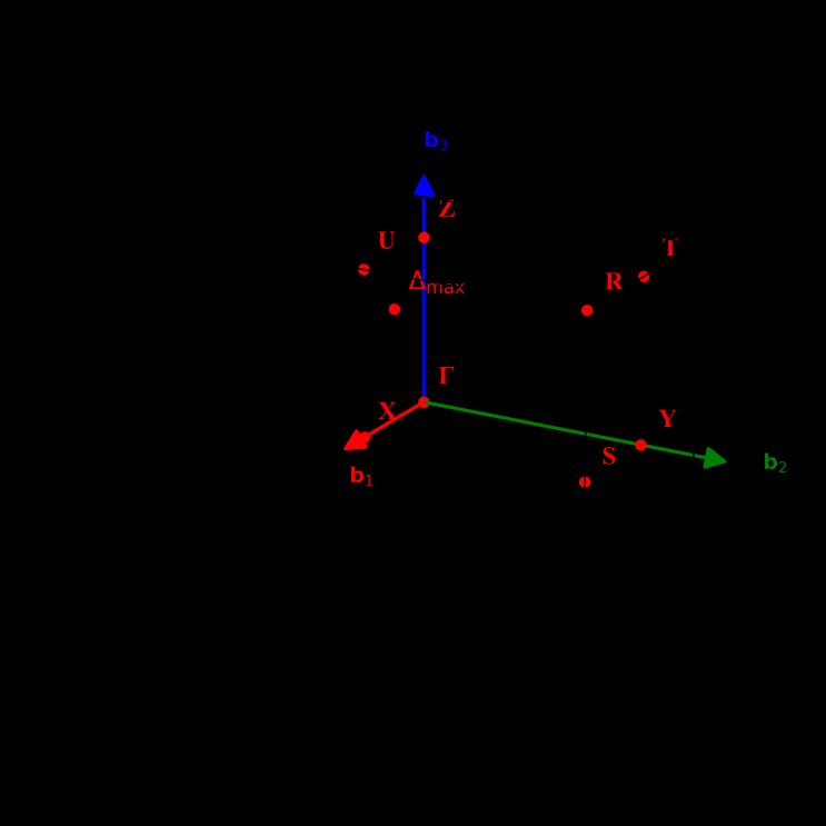
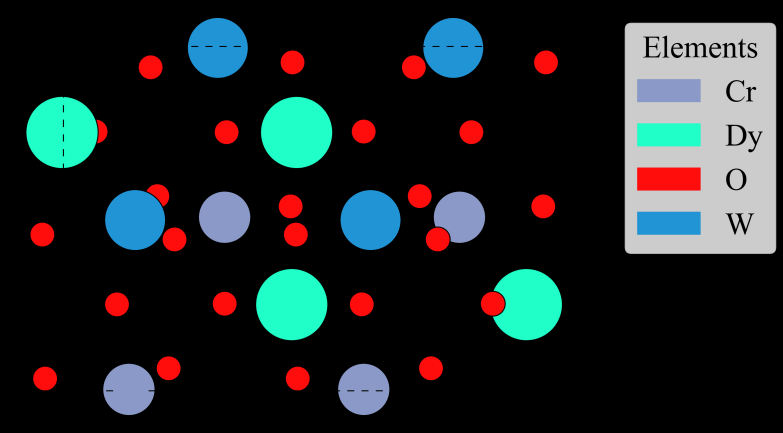
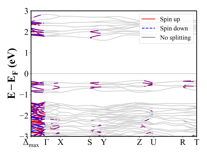
DyFeO3 (Pnma) | Band Gap = 2.861 eV
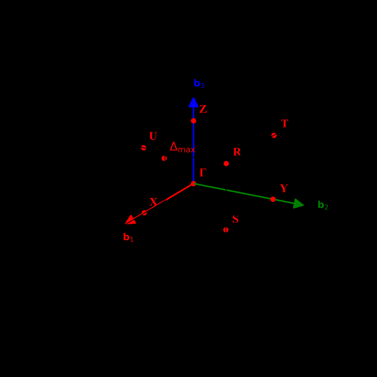
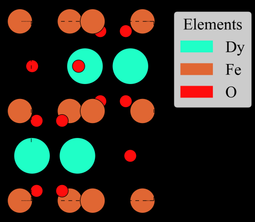
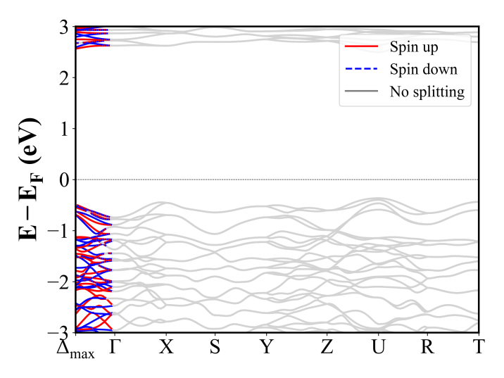
Fe2SiO4 (Pnma) | Band Gap = 2.940 eV
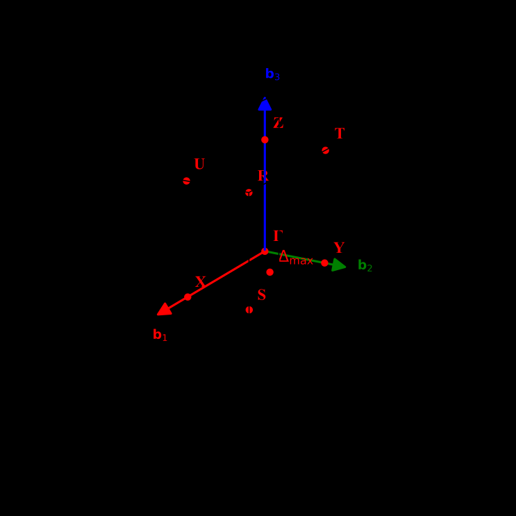
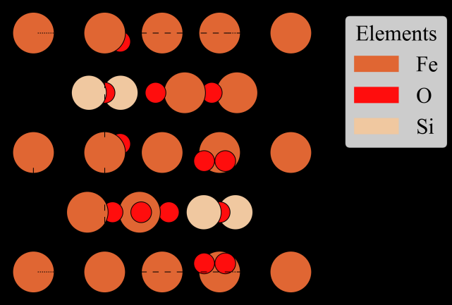
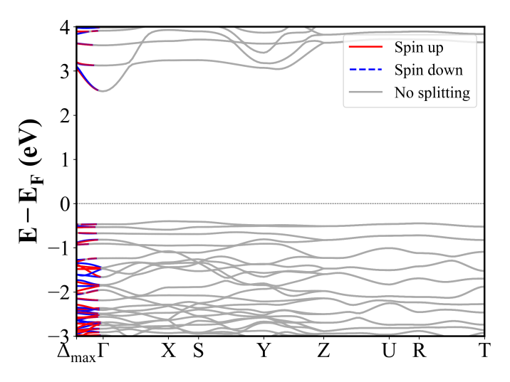
Fe4O5 (Cmcm) | Band Gap = 0.000 eV
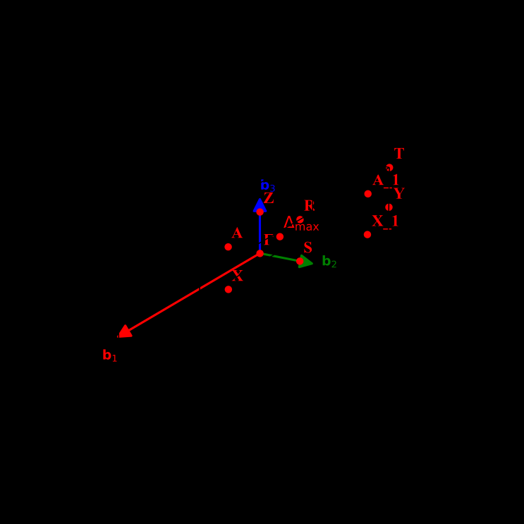
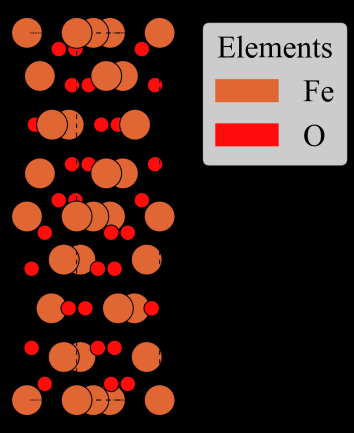
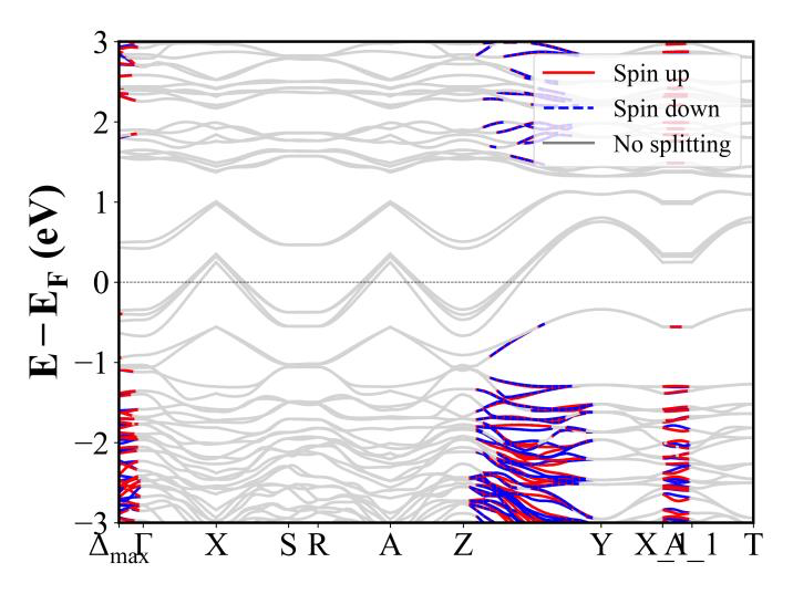
Fe3H4(OF4)2 (C2/m) | Band Gap = 1.706 eV
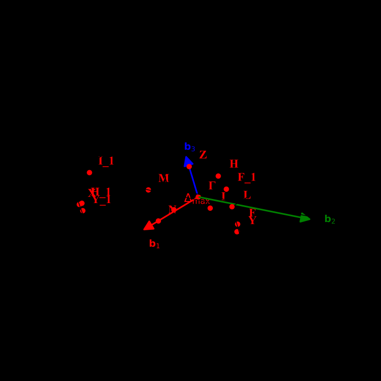
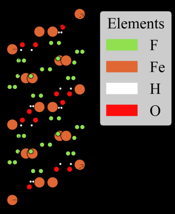
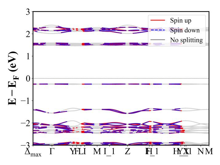
Fe3P2(HO5)2 (P2_1/c) | Band Gap = 2.051 eV
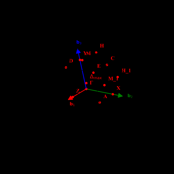
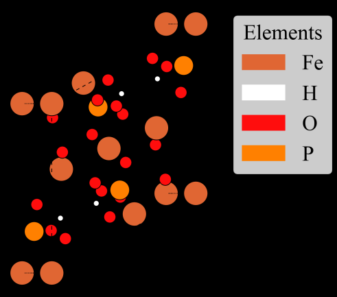
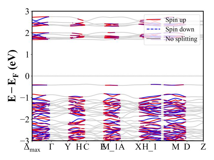
Fe2O3 (R-3c) | Band Gap = 2.566 eV
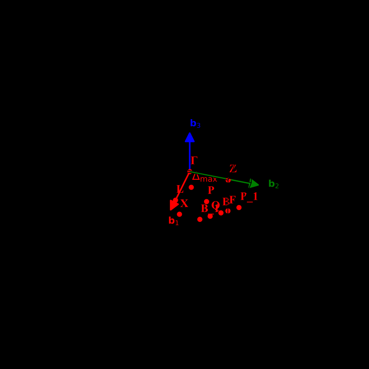
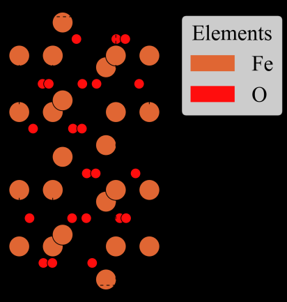
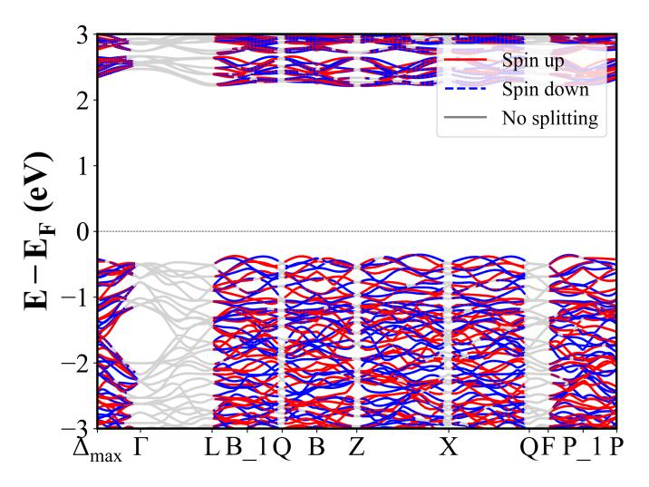
Er2Ru2O7 (Fd-3m) | Band Gap = 0.412 eV
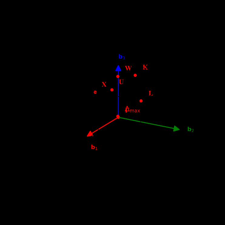
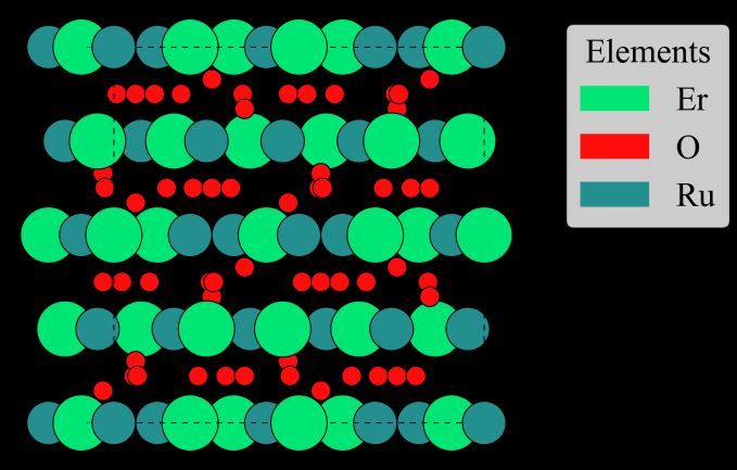
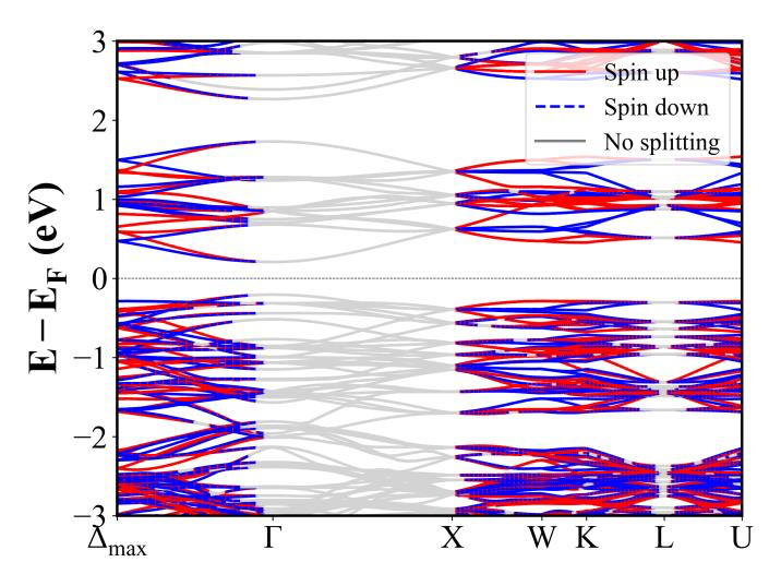
Mn(C2N3)2 (Pnnm) | Band Gap = 3.742 eV
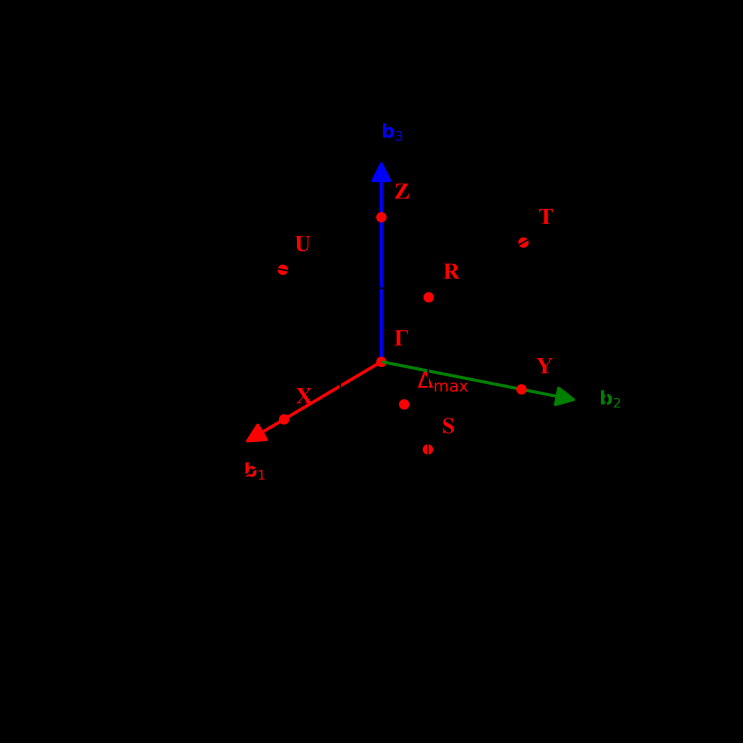
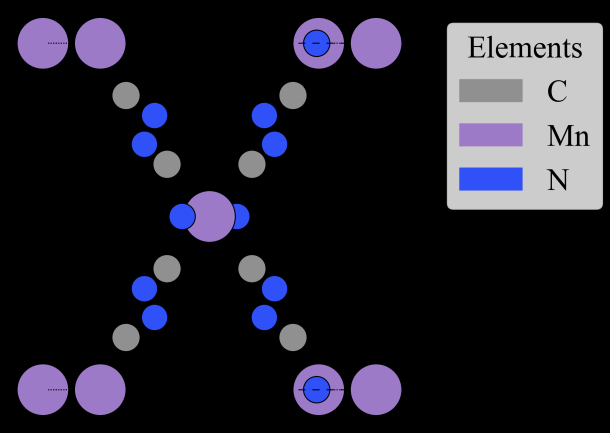
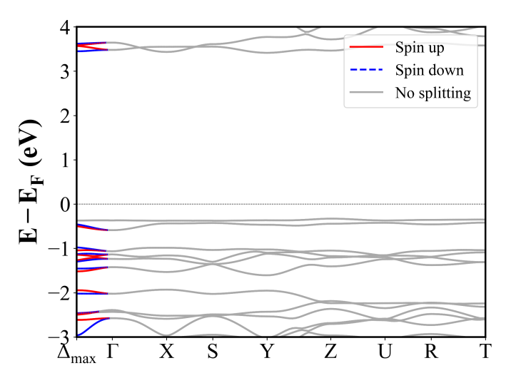
FeBO3 (R-3c) | Band Gap = 2.660 eV
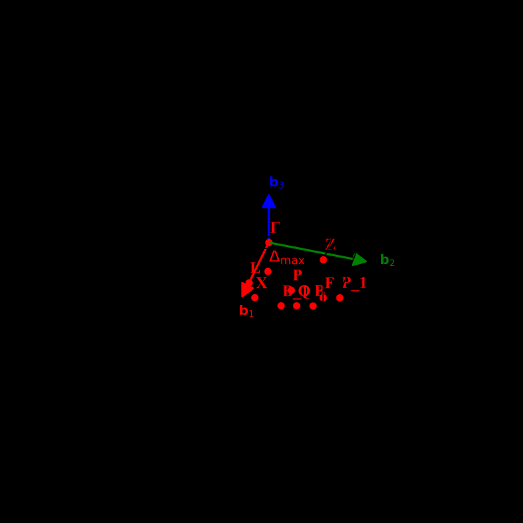
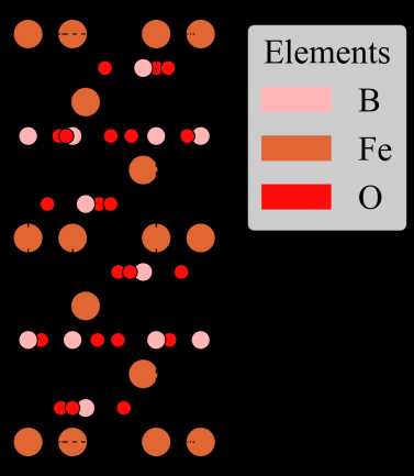
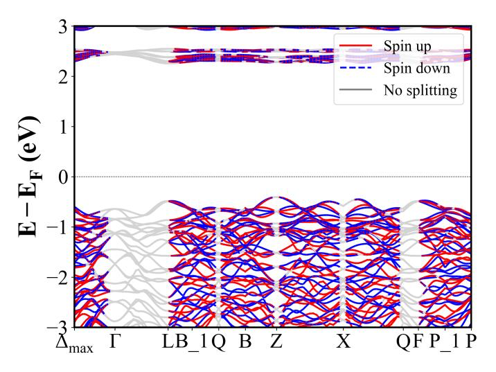
Fe2PO5 (Pnma) | Band Gap = 2.086 eV
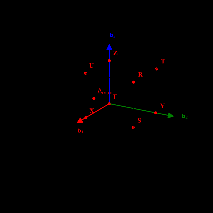
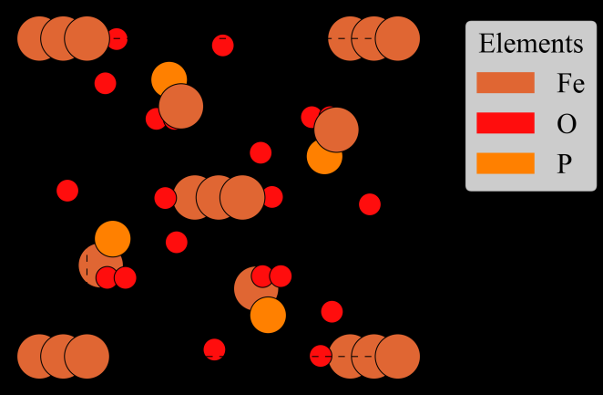
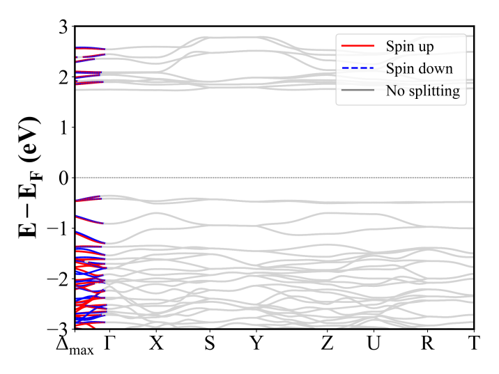
ErVO3 (Pnma) | Band Gap = 1.971 eV
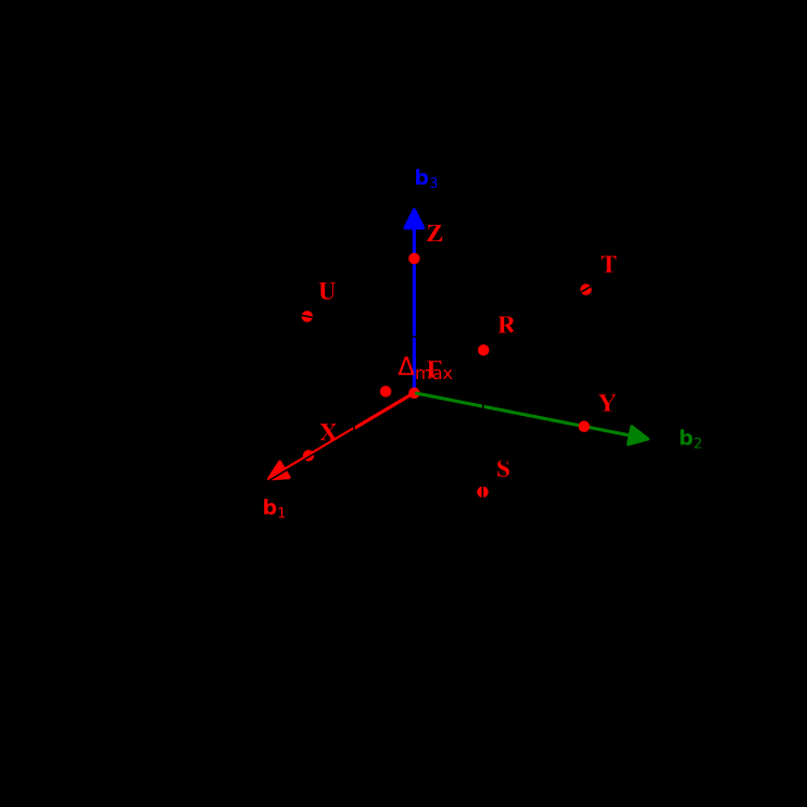
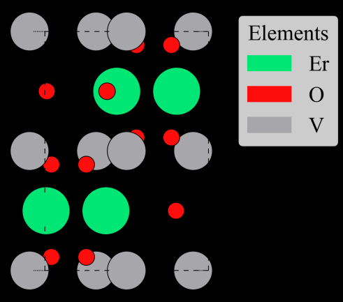
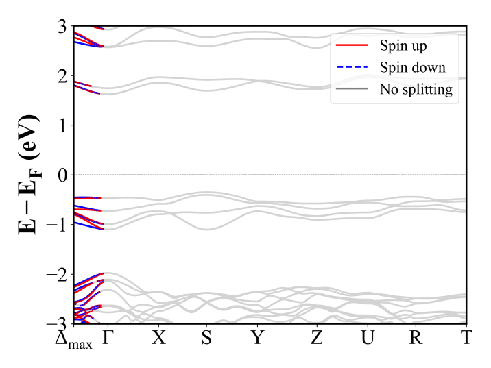
ErCrO3 (Pnma) | Band Gap = 3.143 eV
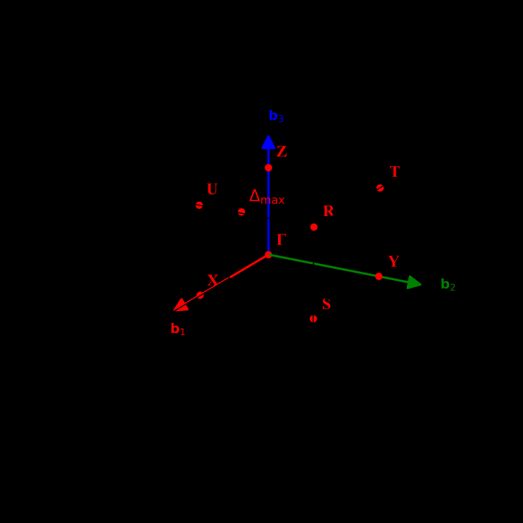
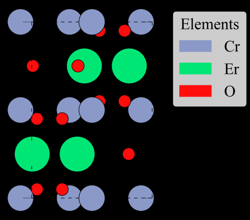
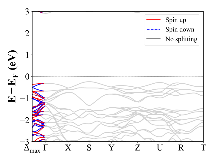
Fe2WO6 (Pbcn) | Band Gap = 1.465 eV
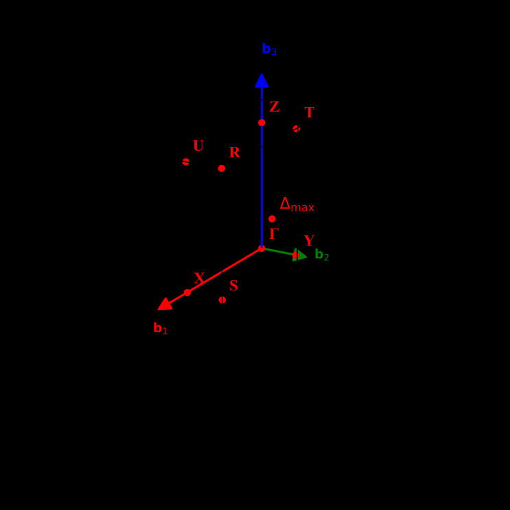
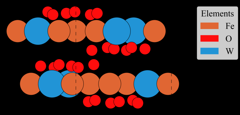
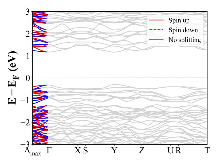
Fe2Mo3O8 (P6_3mc) | Band Gap = 0.000 eV
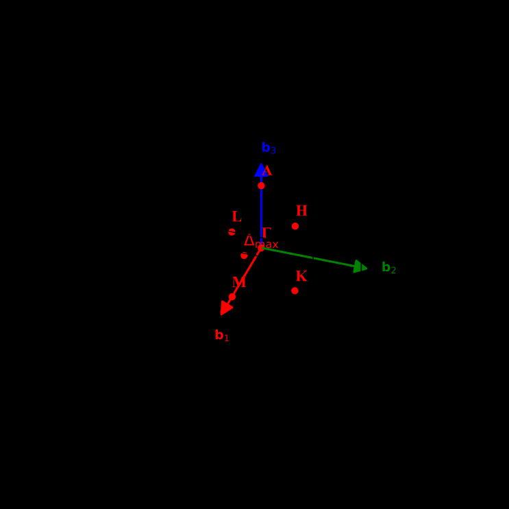
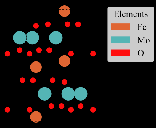
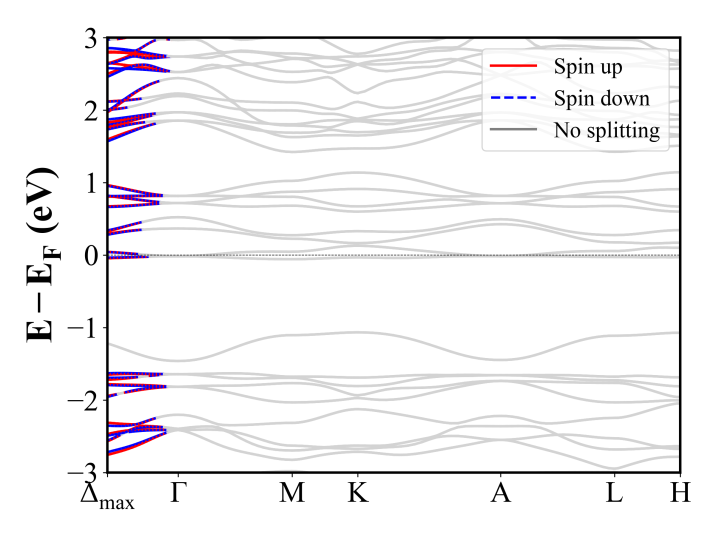
FeSO4F (C2/c) | Band Gap = 2.451 eV
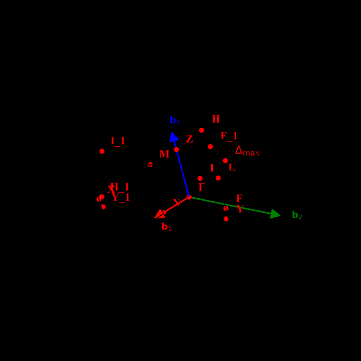
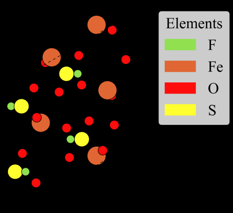
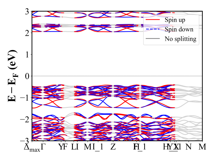
FeF3 (P6_3/m) | Band Gap = 3.764 eV
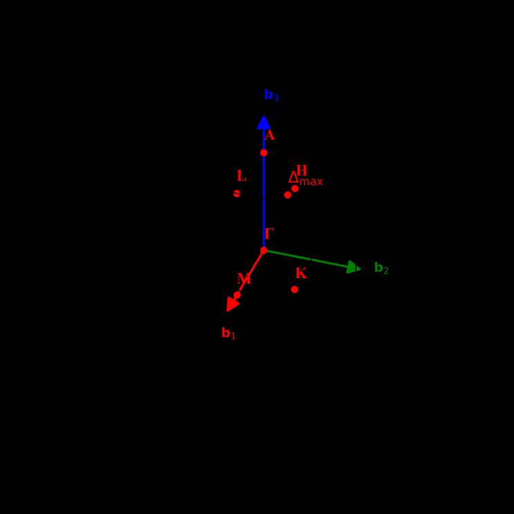
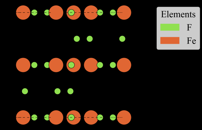
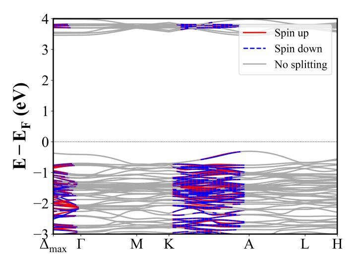
LaCrO3 (R-3c) | Band Gap = 3.194 eV
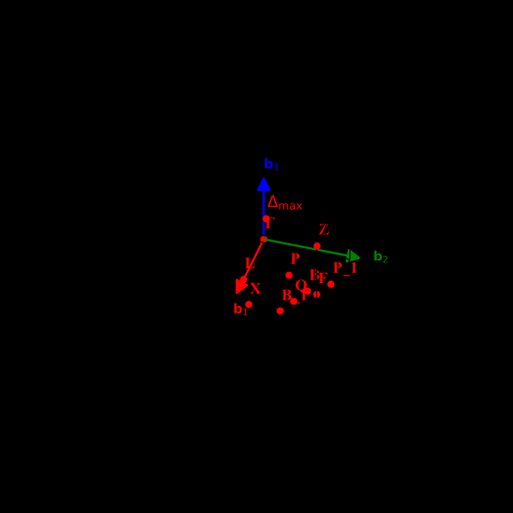
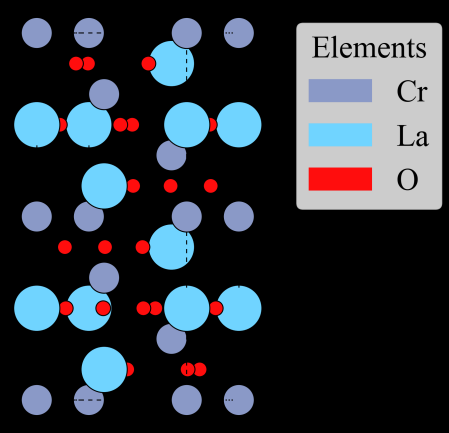
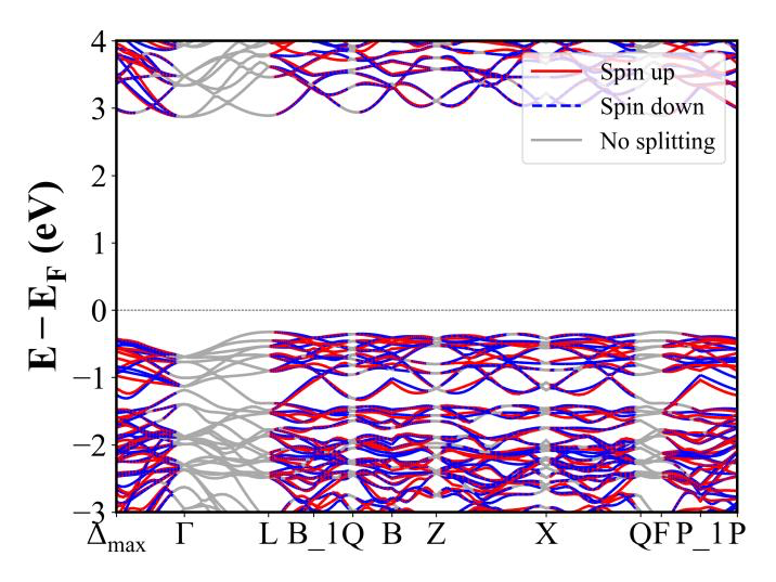
HoMnO3 (P6_3cm) | Band Gap = 1.310 eV
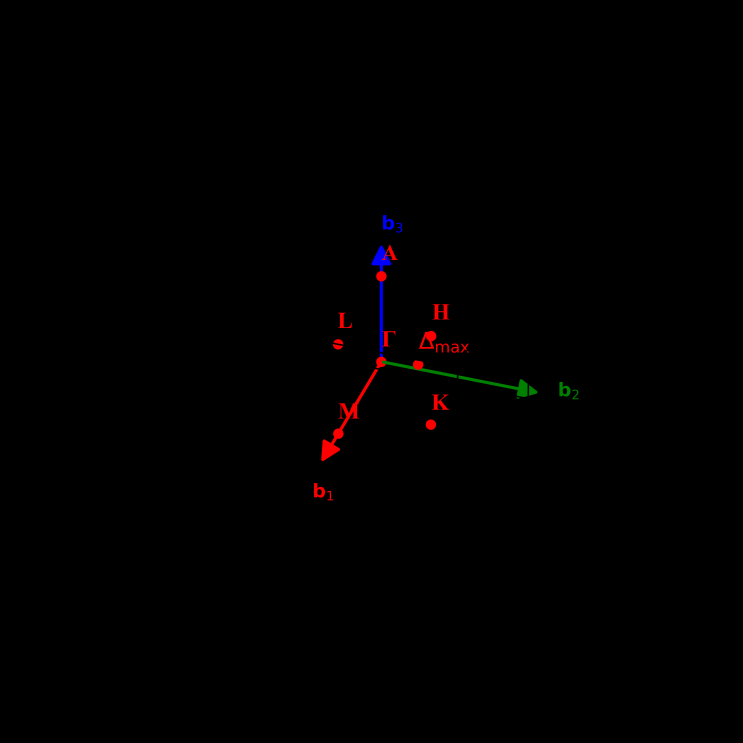
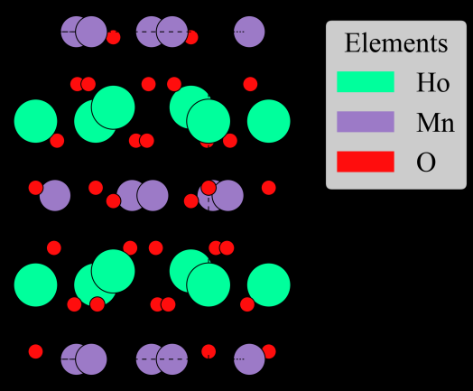
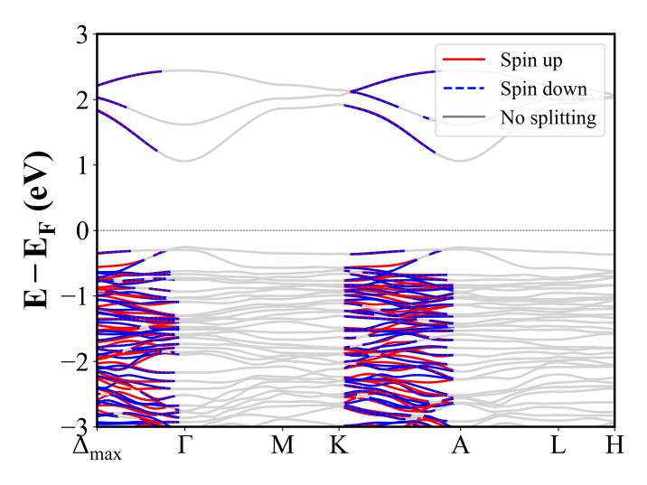
FeF3 (R-3c) | Band Gap = 4.342 eV
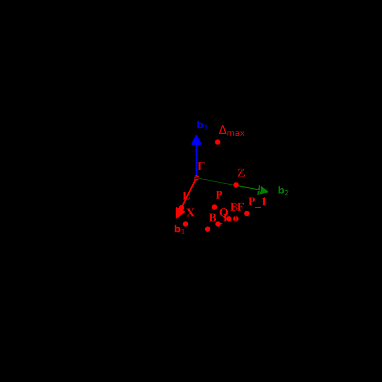
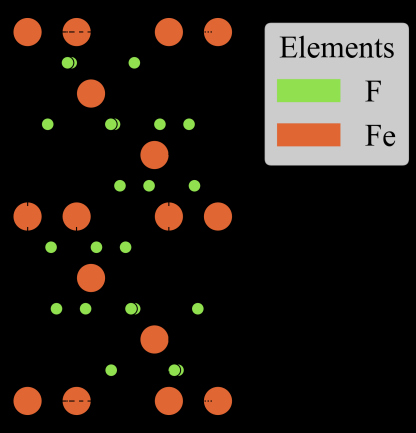
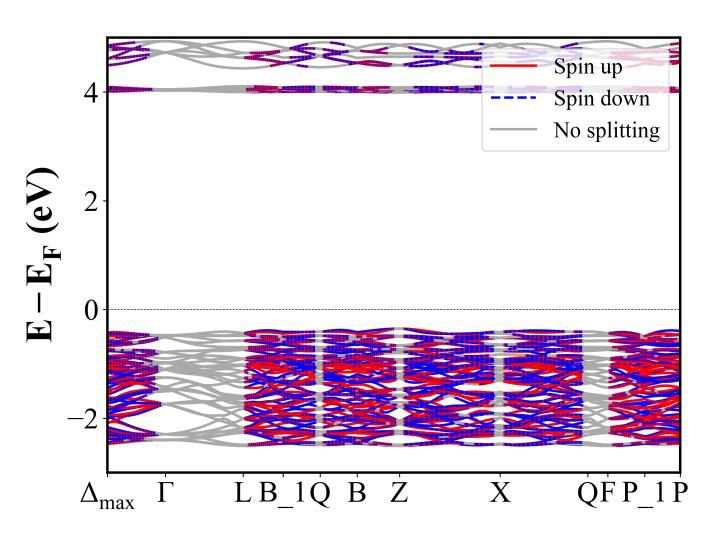
La2NiO4 (P4_2/ncm) | Band Gap = 2.313 eV
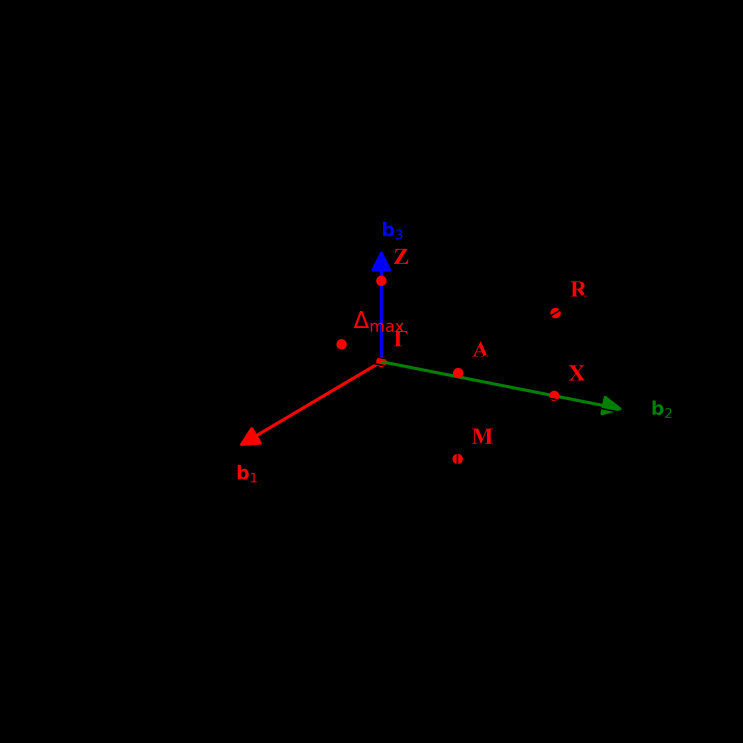
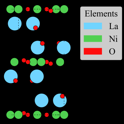
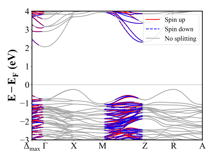
HoFeO3 (Pnma) | Band Gap = 2.735 eV
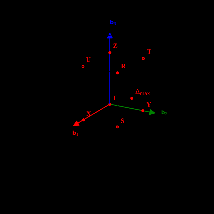
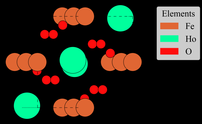
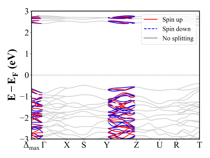
CrInO3 (Pnma) | Band Gap = 1.886 eV
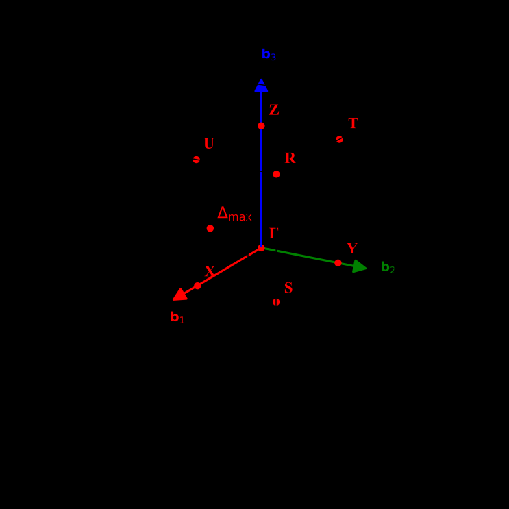
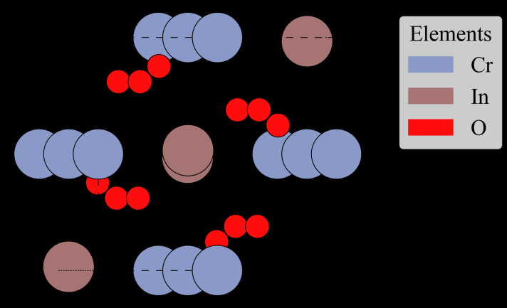
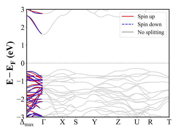
FeCO3 (R-3c) | Band Gap = 3.688 eV

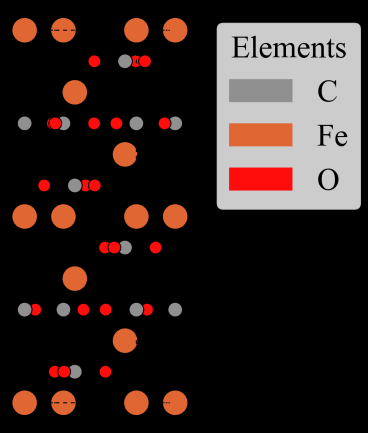
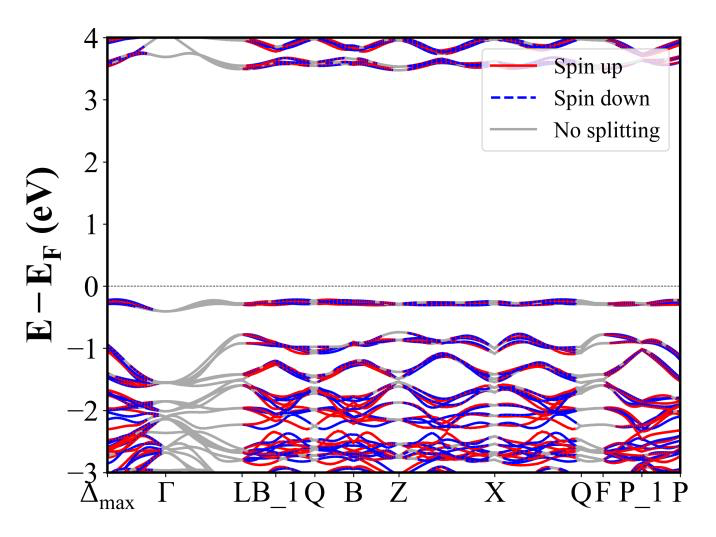
LiLa2RuO6 (P2_1/c) | Band Gap = 1.220 eV
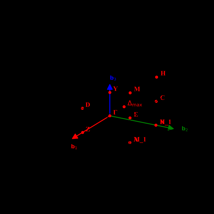
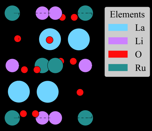
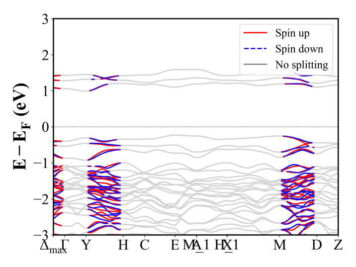
FeHSO5 (C2/c) | Band Gap = 2.625 eV
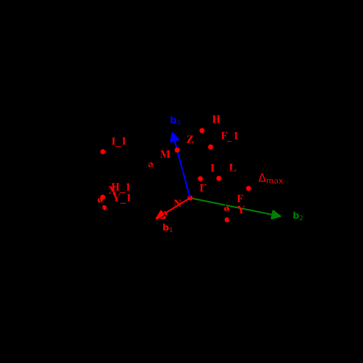
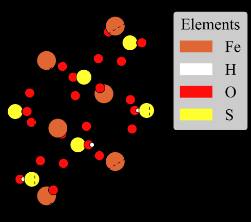
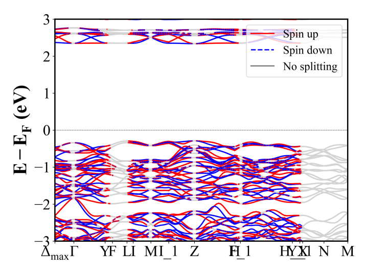
K2ReI6 (P2_1/c) | Band Gap = 1.483 eV
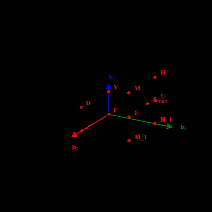
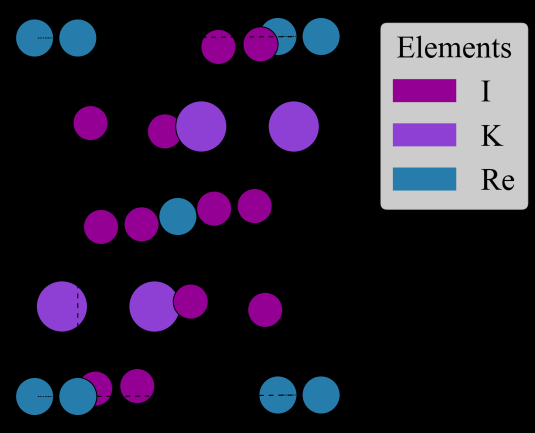
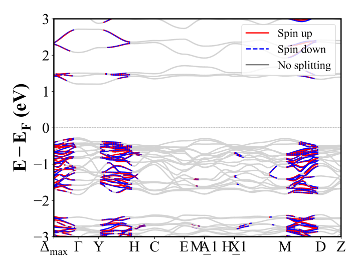
LaCrO3 (Pnma) | Band Gap = 3.105 eV
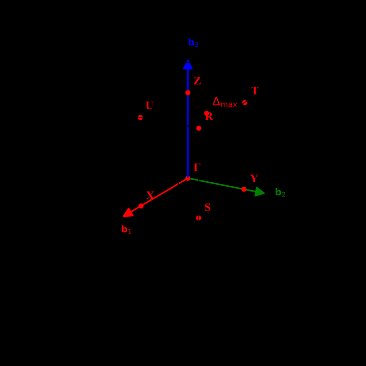
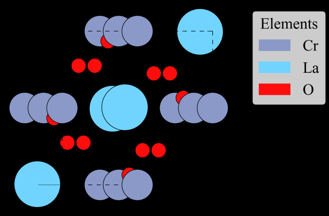
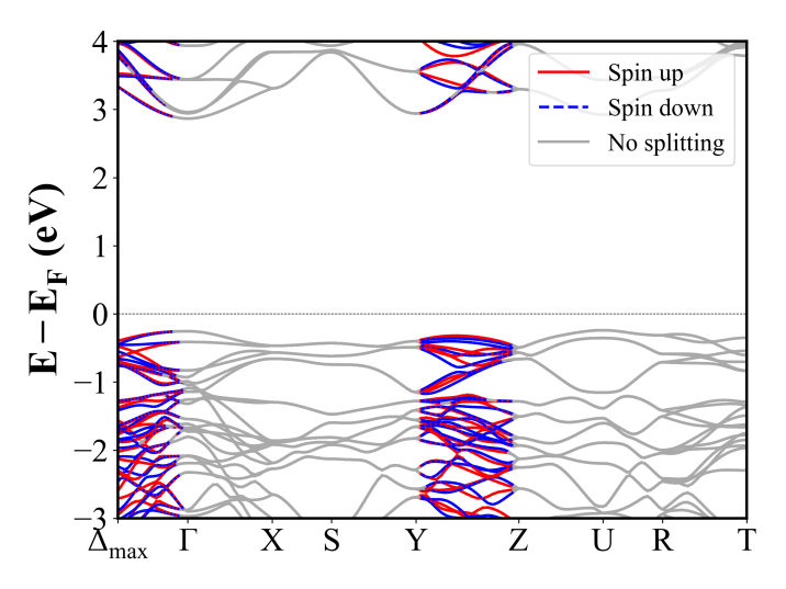
La2CoIrO6 (P2_1/c) | Band Gap = 0.000 eV
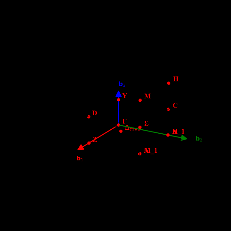
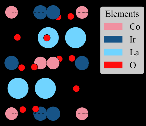
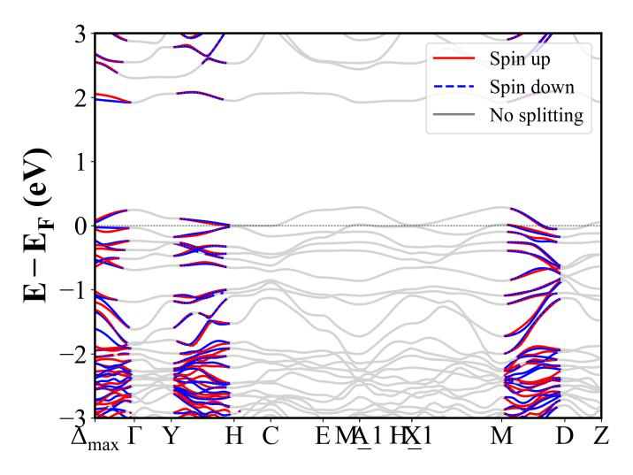
HoCrWO6 (Pna2_1) | Band Gap = 2.398 eV
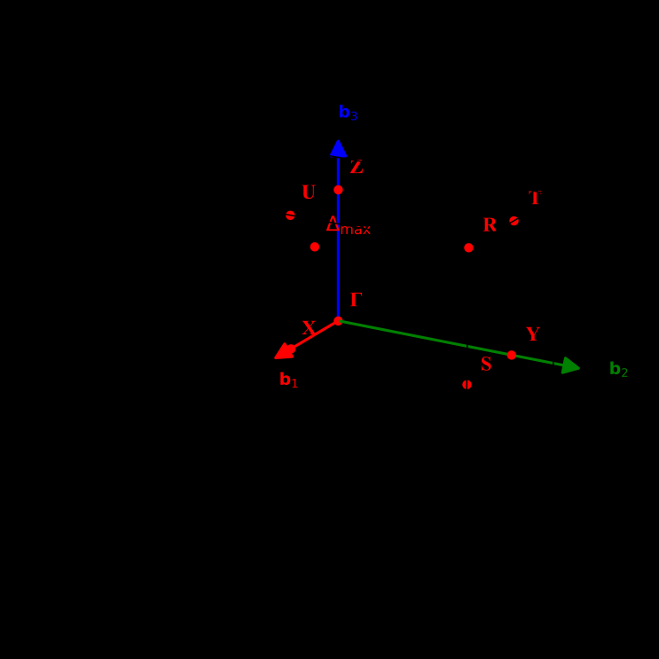
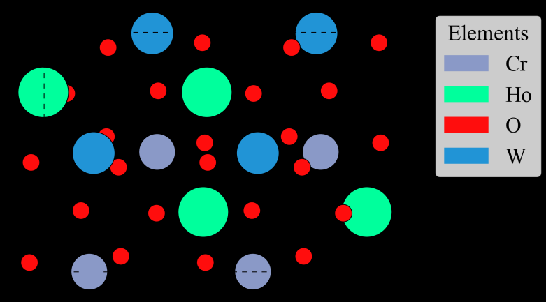
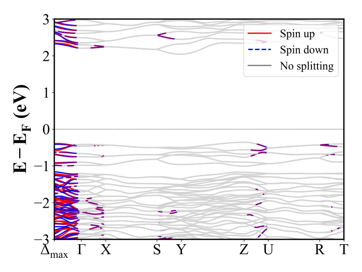
LiFeP2O7 (P2_1) | Band Gap = 2.958 eV
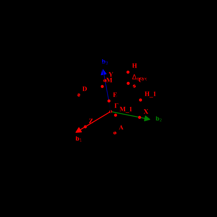
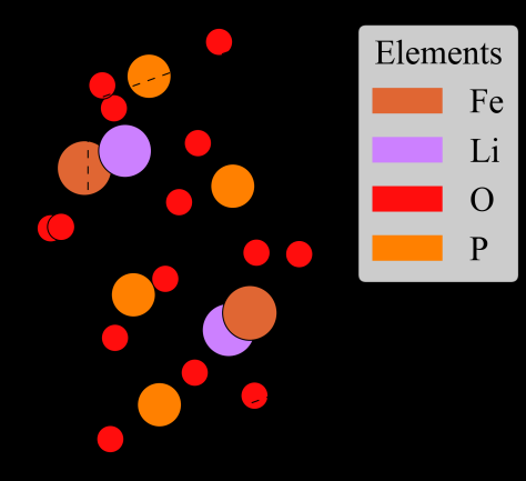
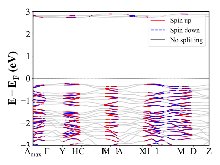
Li2Co(SO4)2 (P2_1/c) | Band Gap = 3.224 eV
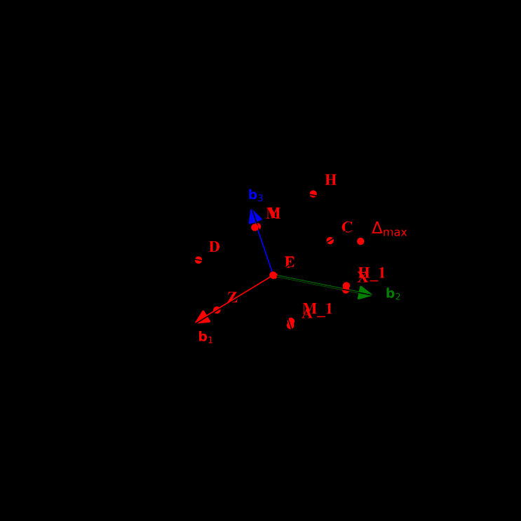
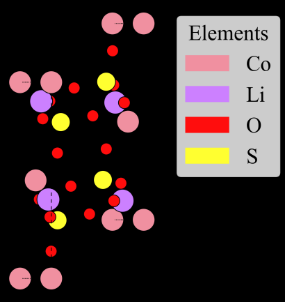
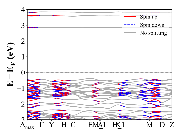
MnSiN2 (Pna2_1) | Band Gap = 2.733 eV
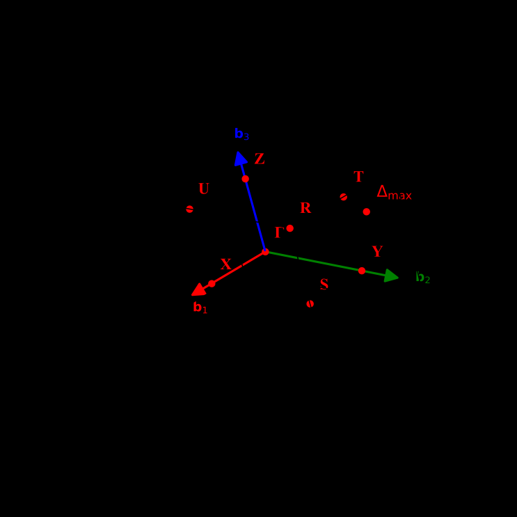
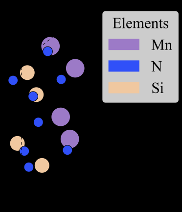
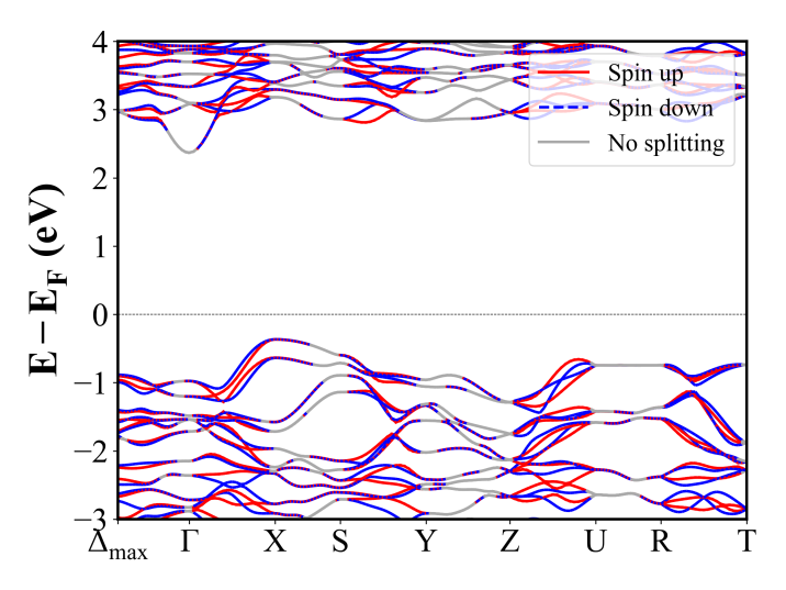
Mn3B7IO13 (Pca2_1)
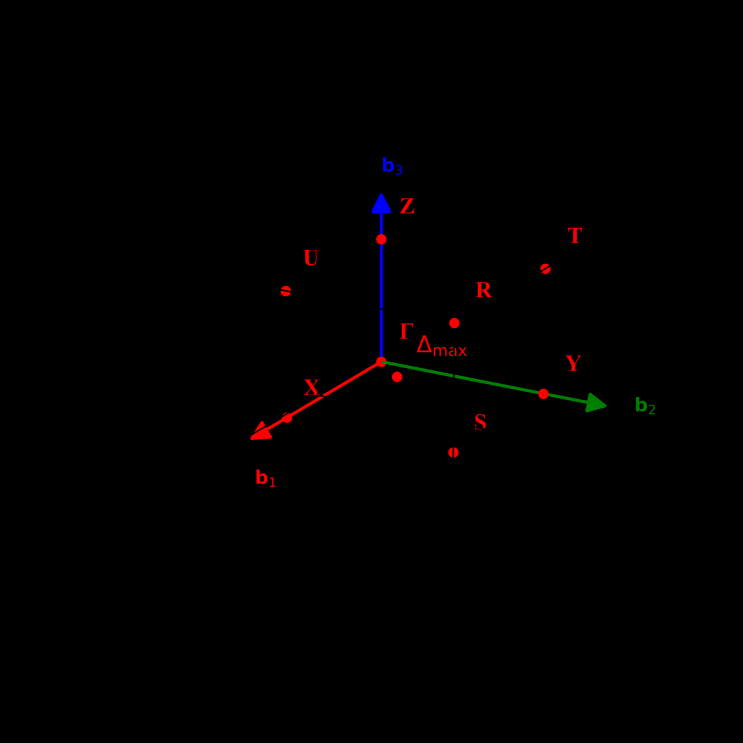
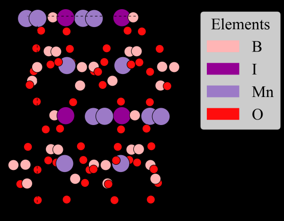
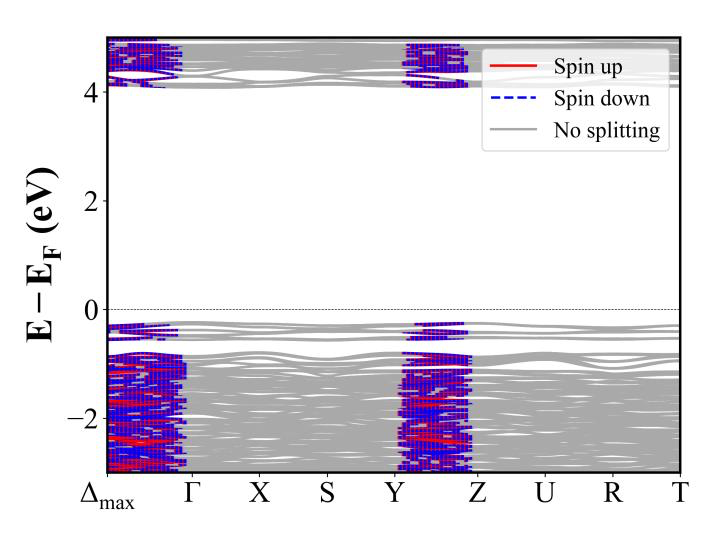
MgCr2O4 (Fd-3m) | Band Gap = 1.545 eV
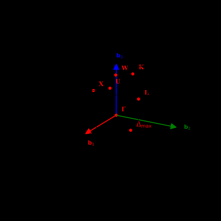
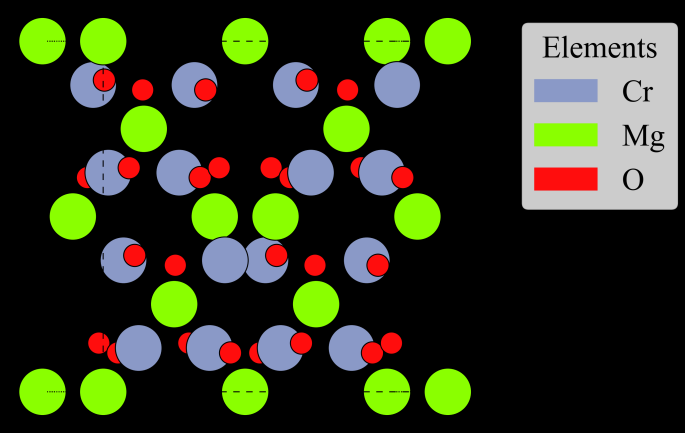
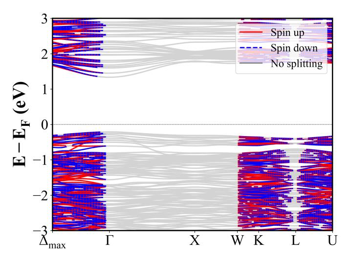
LaMnO3 (Pnma) | Band Gap = 1.237 eV
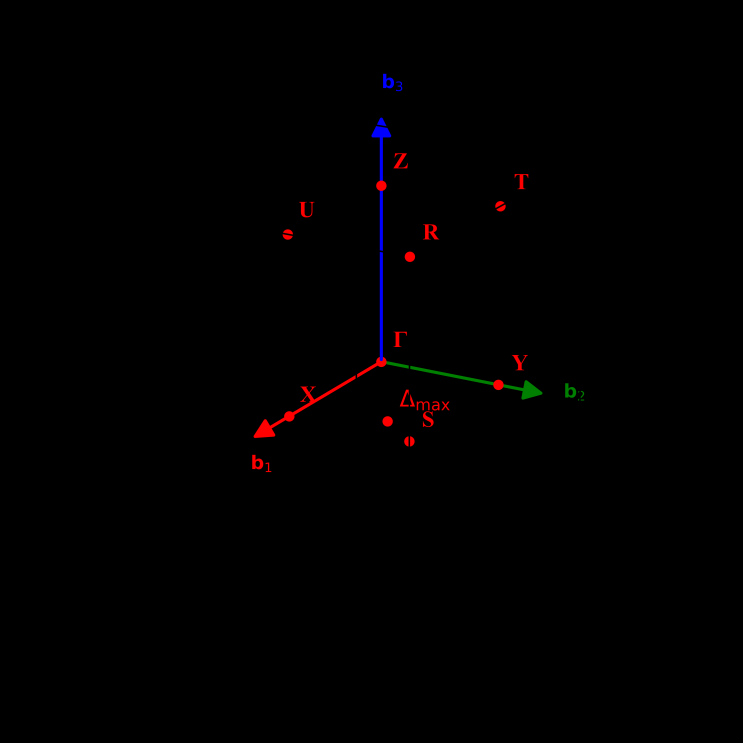
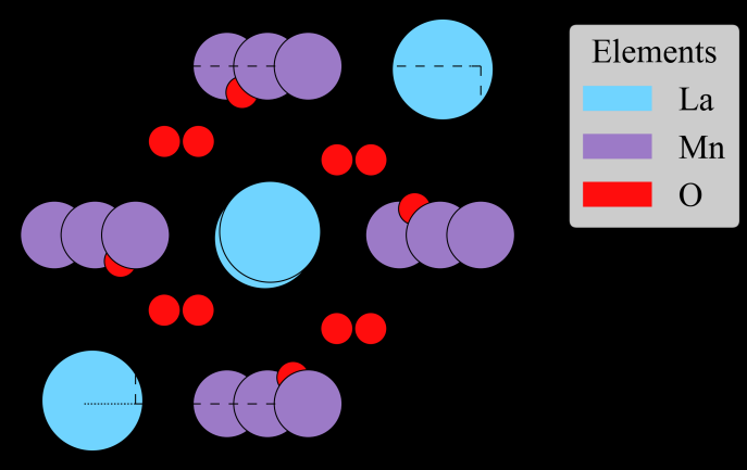
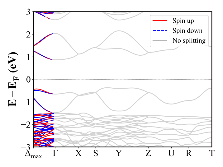
LuCrWO6 (Pna2_1) | Band Gap = 2.347 eV
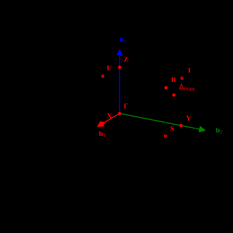
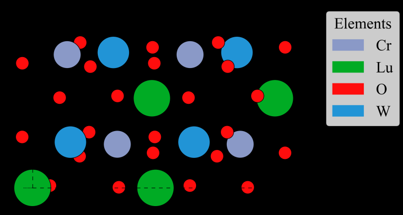
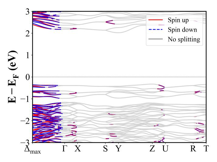
Li2Ni(SO4)2 (P2_1/c) | Band Gap = 4.565 eV
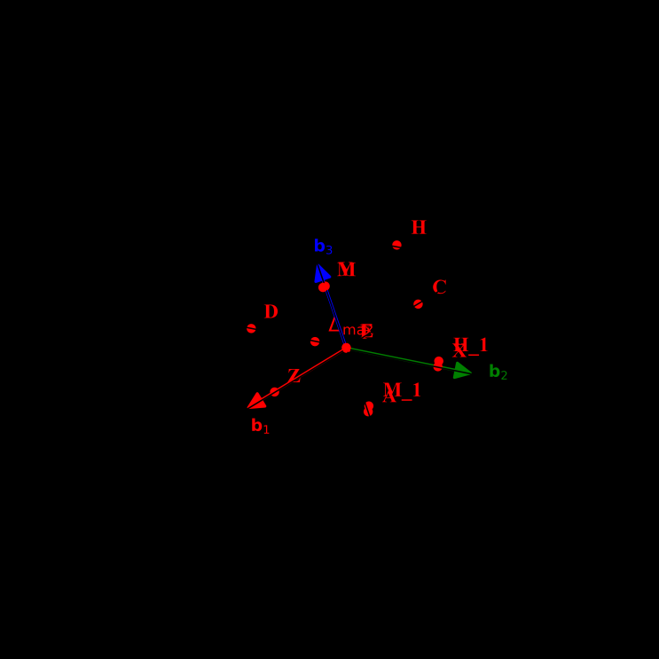
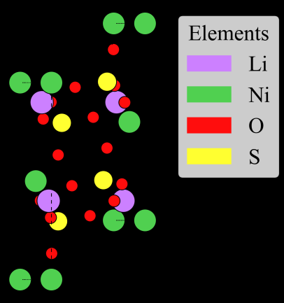
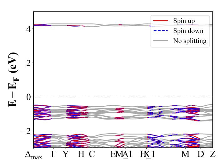
Mn2SeO3F2 (Pnma) | Band Gap = 3.889 eV
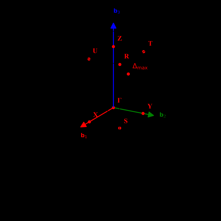
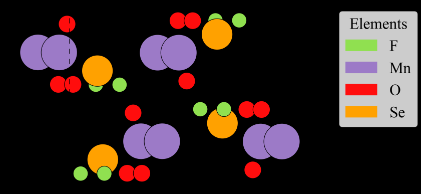
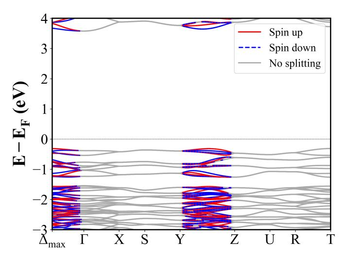
MnF2 (P4_2/mnm) | Band Gap = 3.575 eV
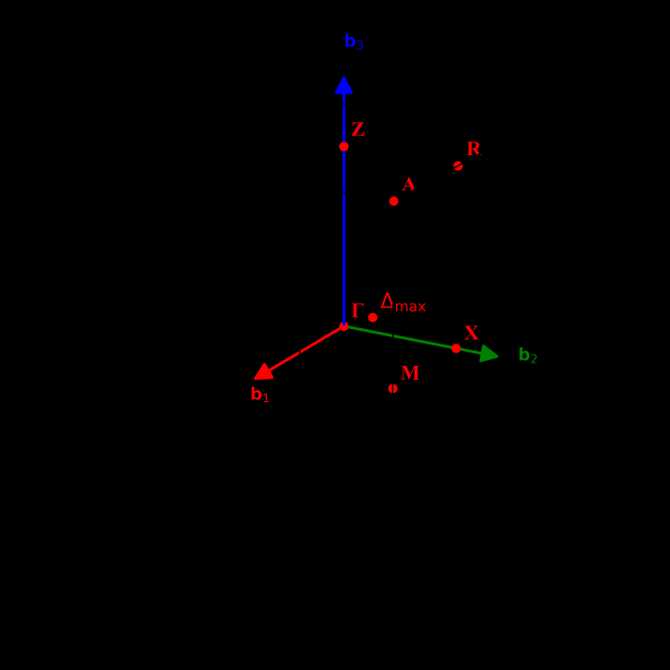
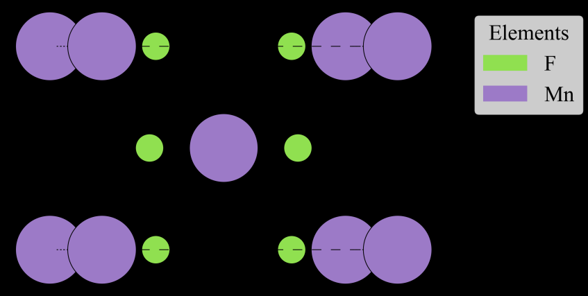
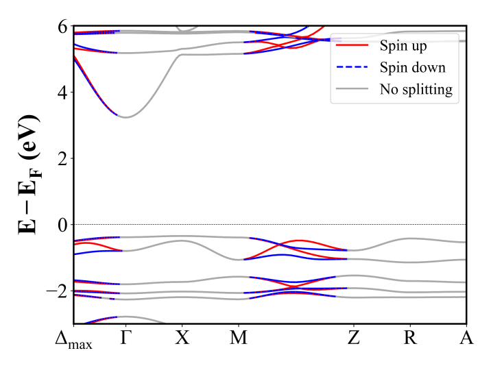
LuFeO3 (P6_3cm) | Band Gap = 1.795 eV
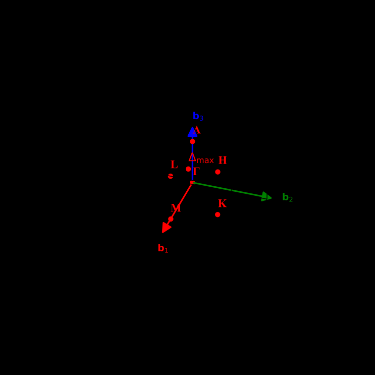
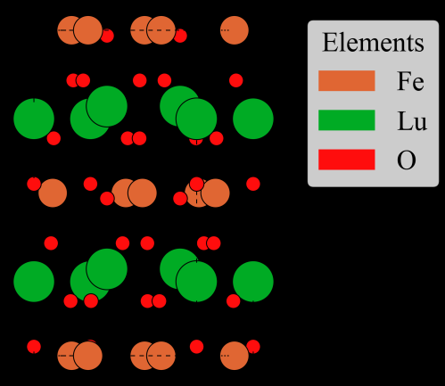
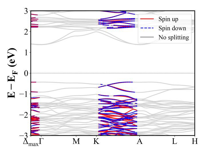
MnSe2 (Pa-3) | Band Gap = 0.983 eV
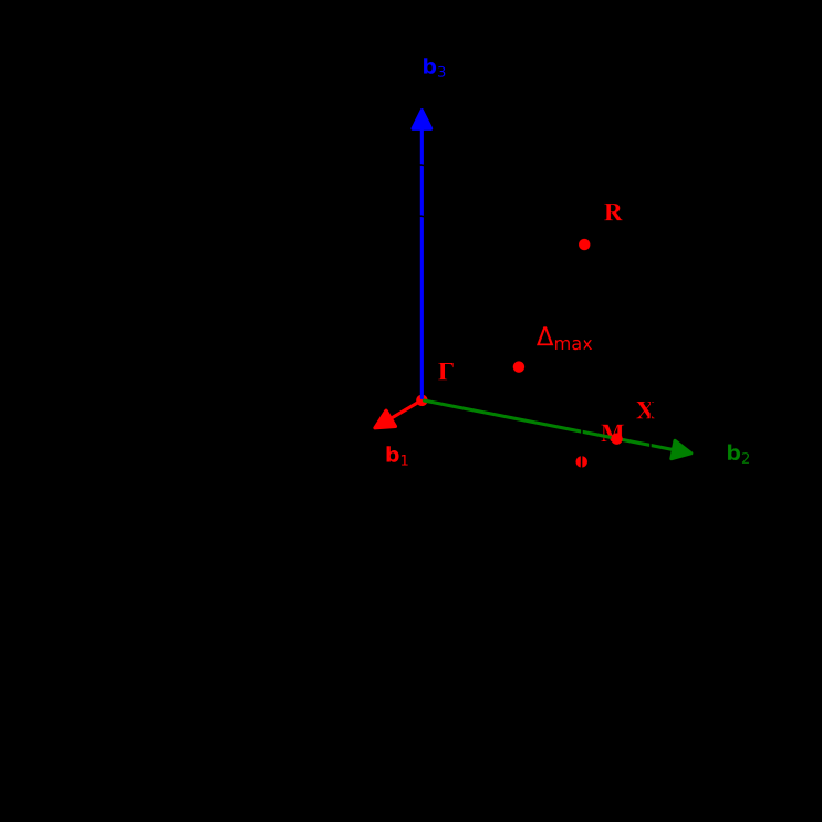
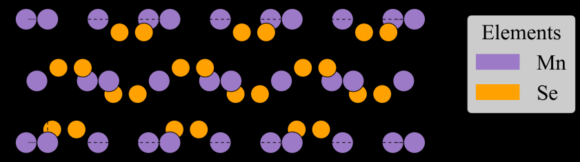
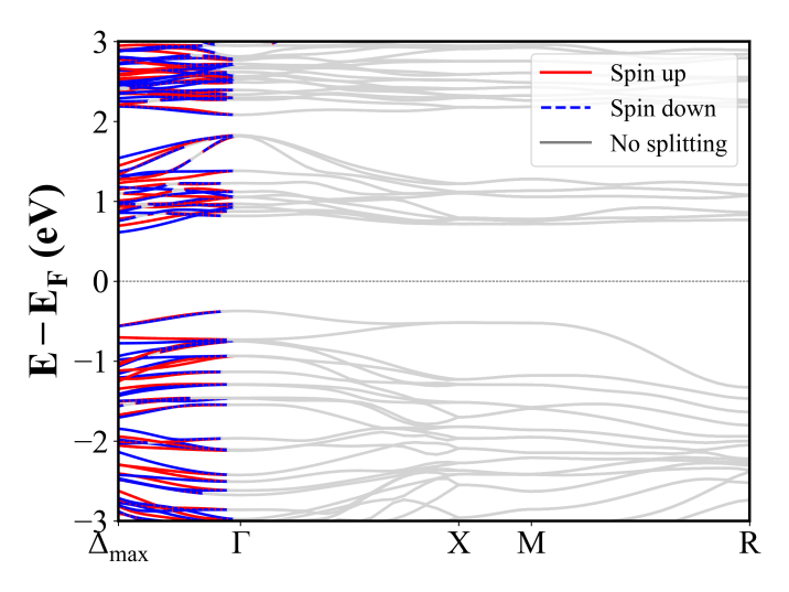
Mn(C2N3)2 (Pnnm) | Band Gap = 4.076 eV
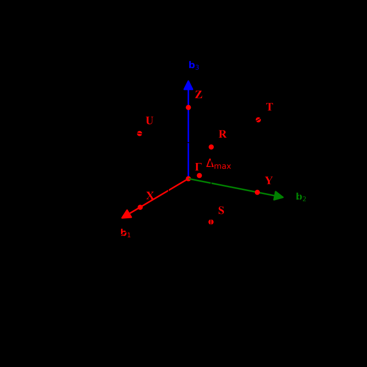
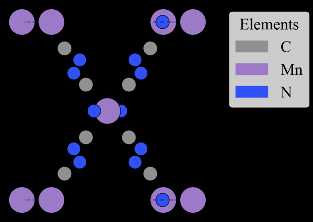
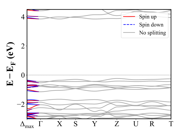
Mn2O3 (Pbca) | Band Gap = 0.946 eV
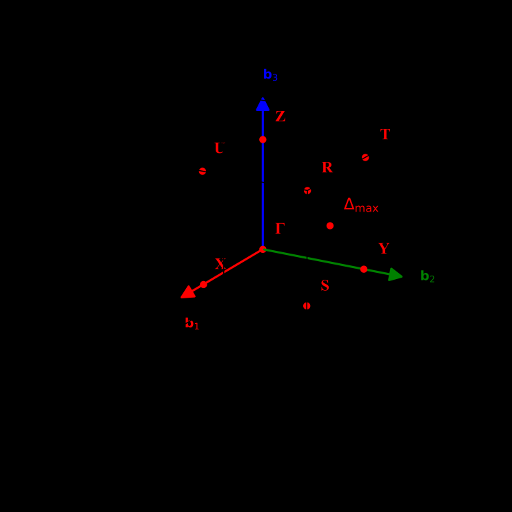
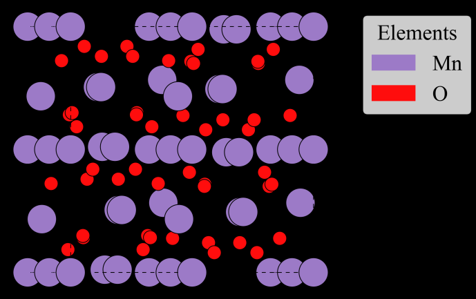
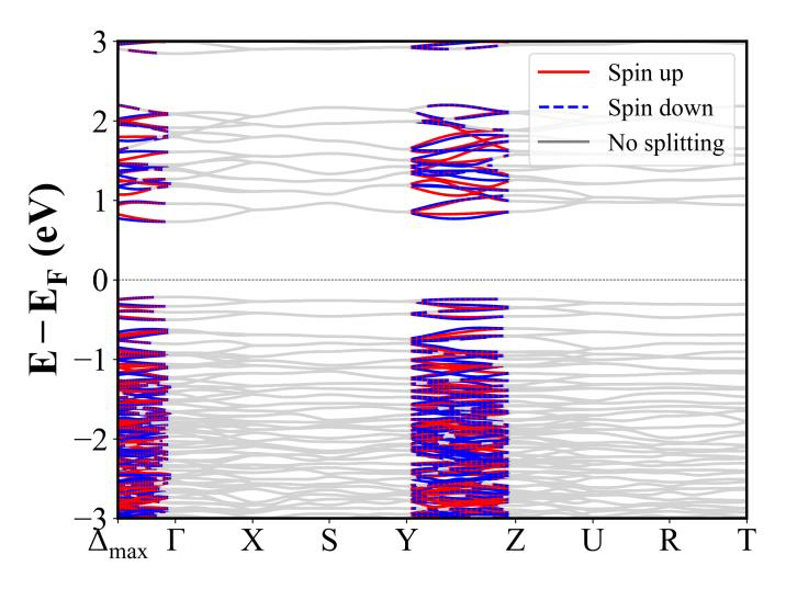
MnGeN2 (Pna2_1) | Band Gap = 1.516 eV
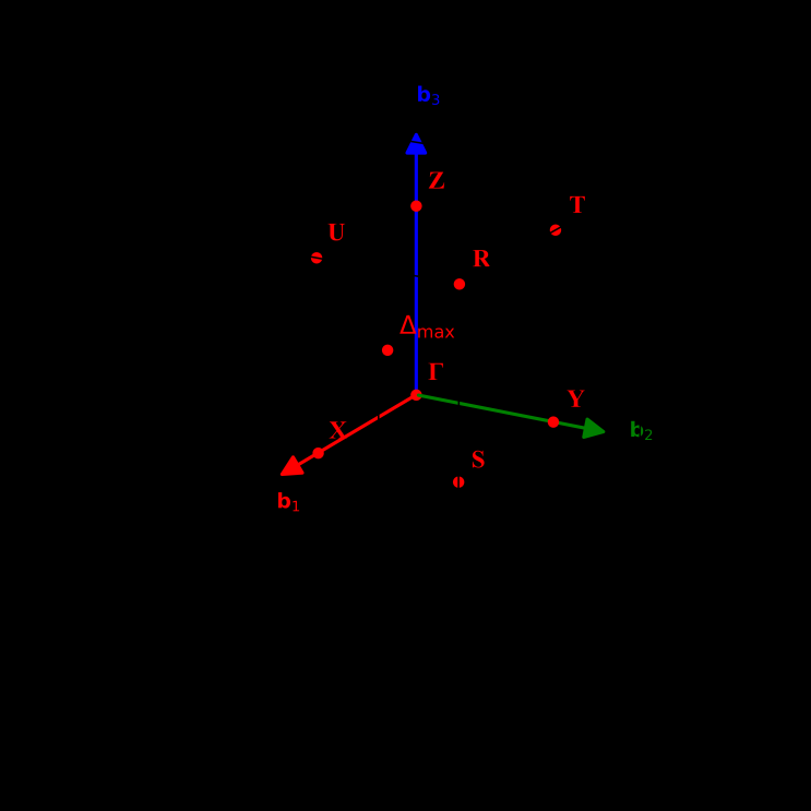
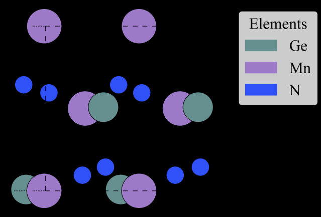
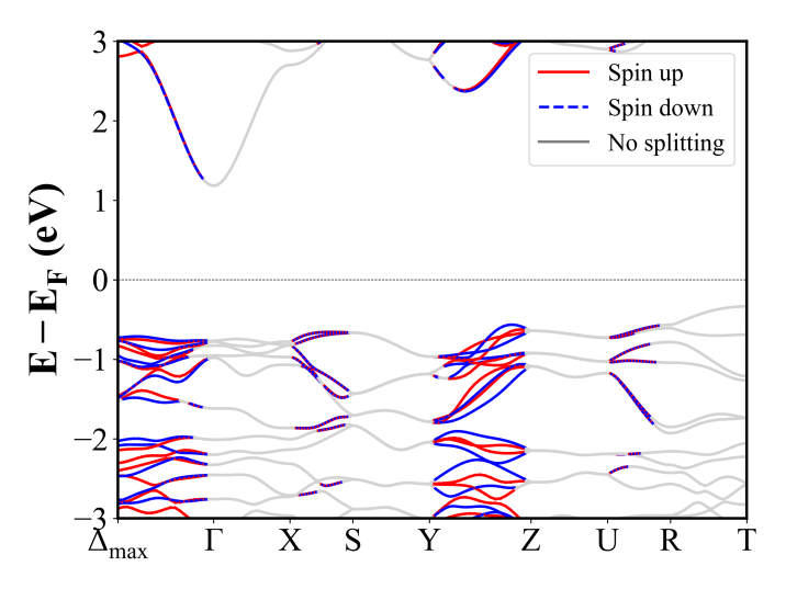
MnCO3 (R-3c) | Band Gap = 4.015 eV
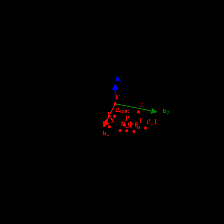
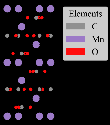
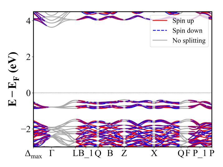
Mn4Nb2O9 (Cc) | Band Gap = 1.270 eV
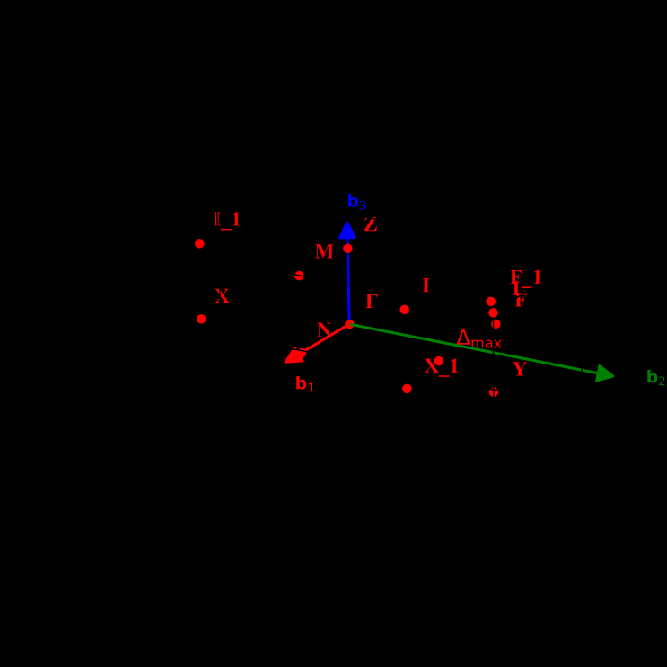
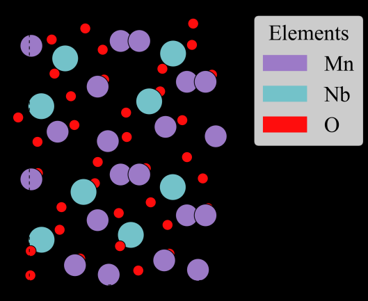
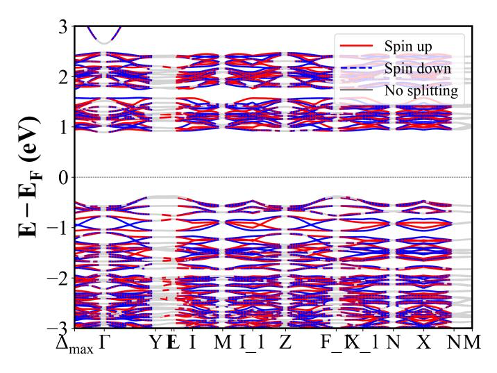
LuCrO3 (Pnma) | Band Gap = 3.192 eV
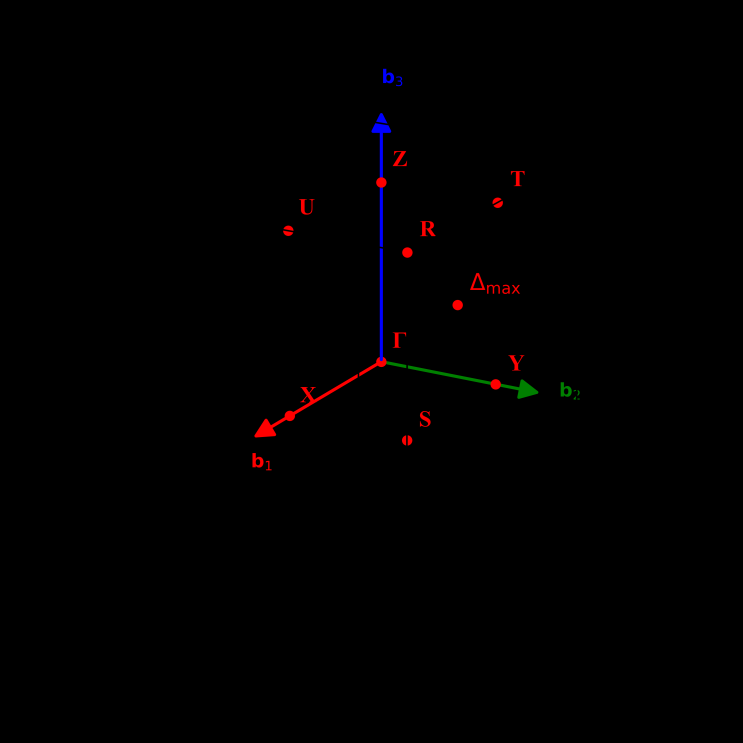
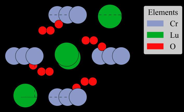
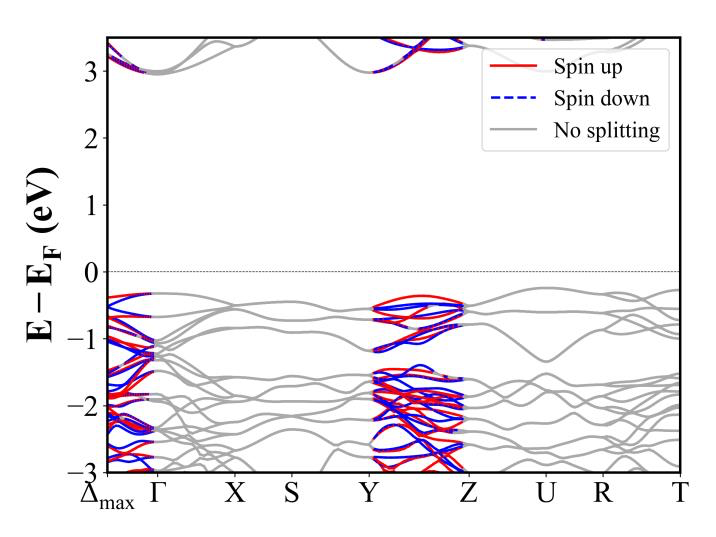
Li2Mn(SO4)2 (P2_1/c) | Band Gap = 5.101 eV
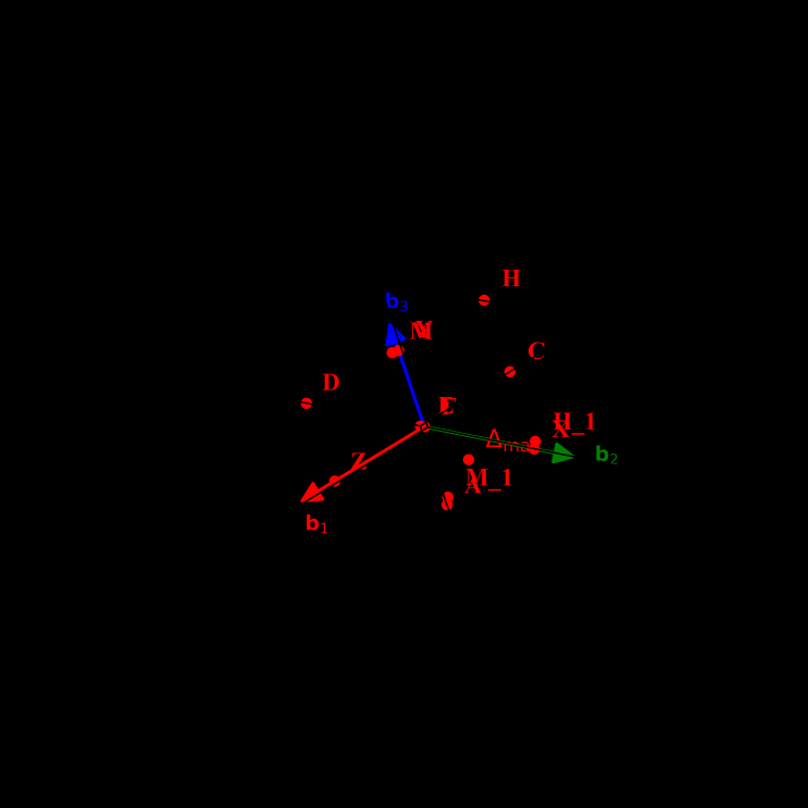
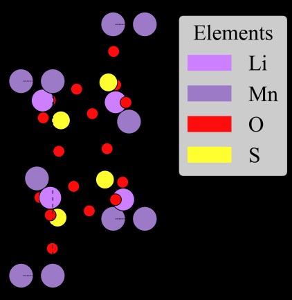
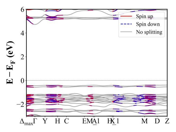
LuVO3 (Pnma) | Band Gap = 1.991 eV
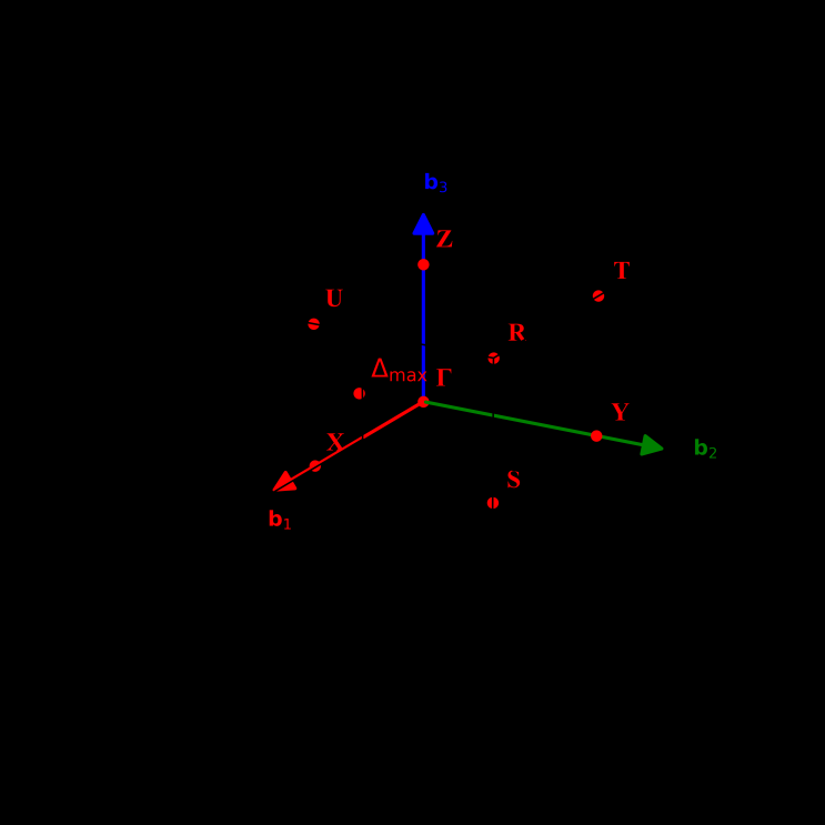
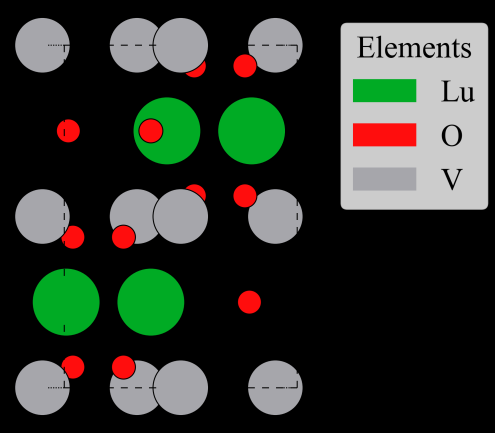
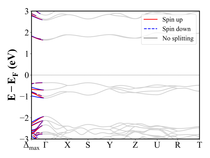
Mn2GeO4 (Pnma) | Band Gap = 0.594 eV
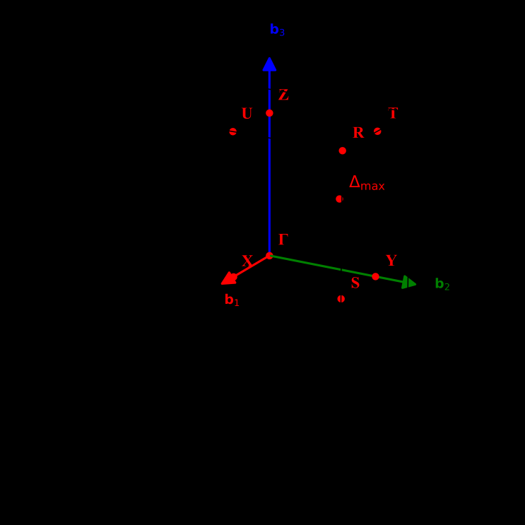
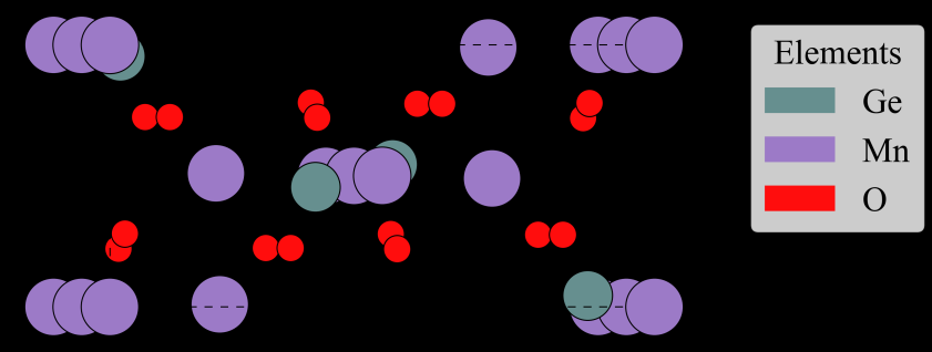
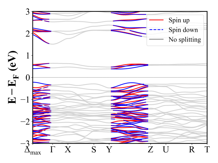
LiFe2F6 (P4_2/mnm) | Band Gap = 0.168 eV
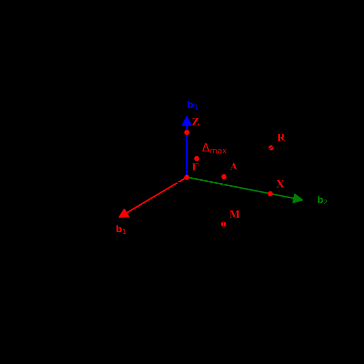
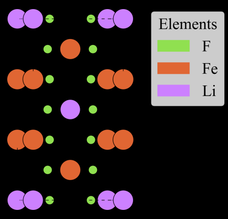
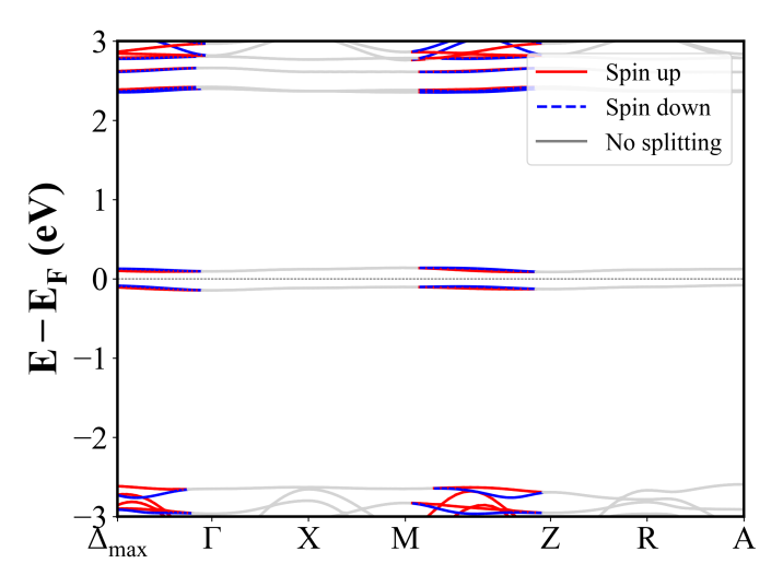
NaOsO3 (Pnma) | Band Gap = 0.103 eV
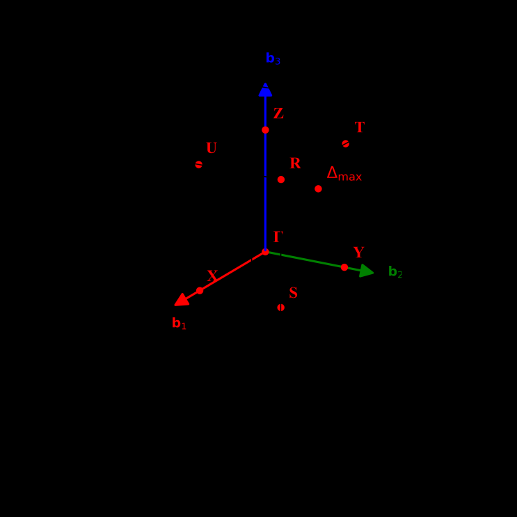
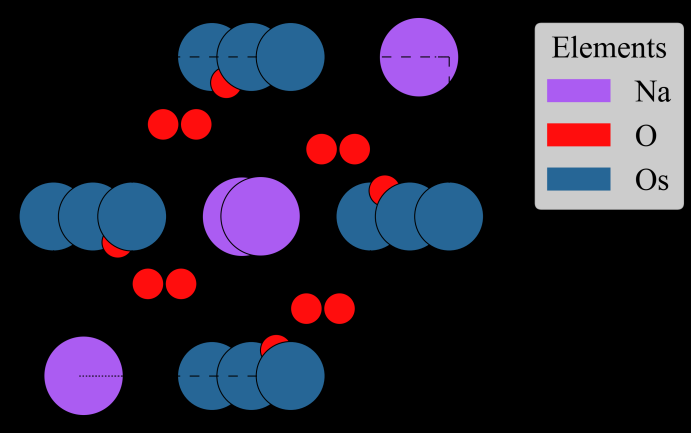
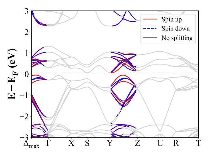
MnTe (P6_3/mmc) | Band Gap = 0.764 eV
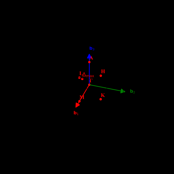
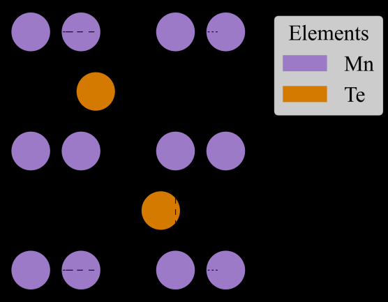
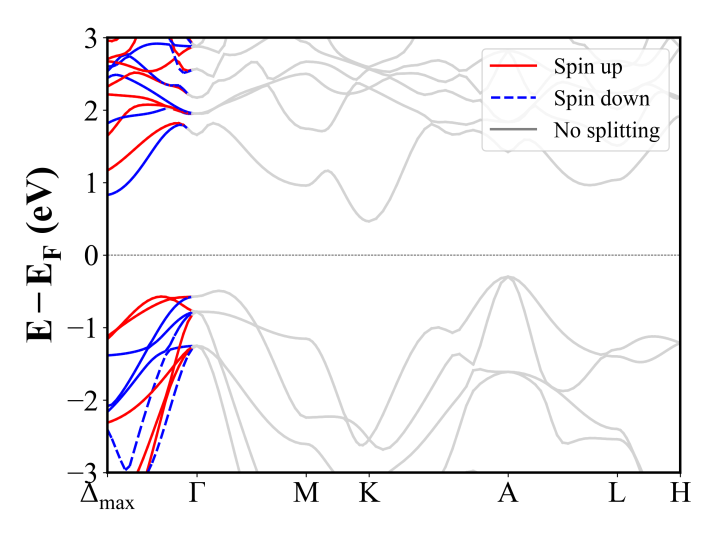
TiMnO3 (R3c) | Band Gap = 2.475 eV
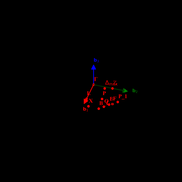
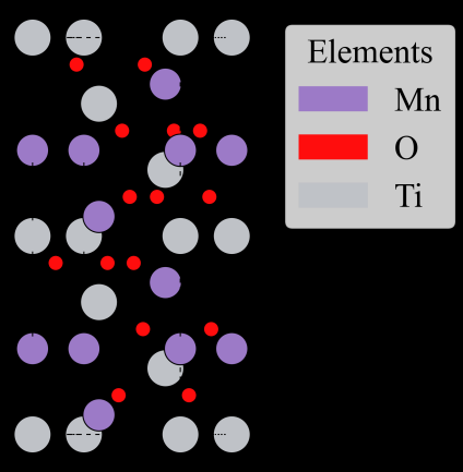
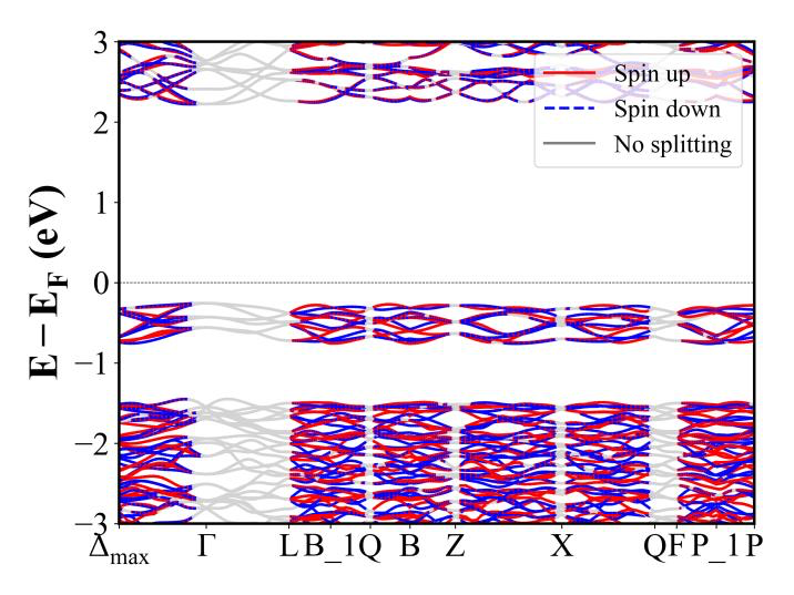
MnNbP (Pnma) | Band Gap = 0.000 eV
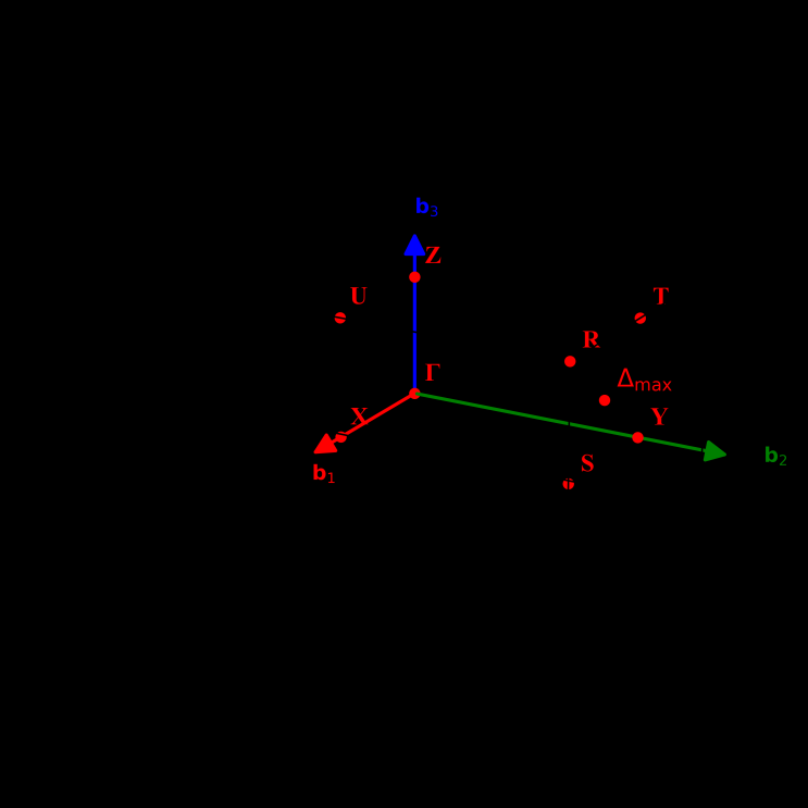
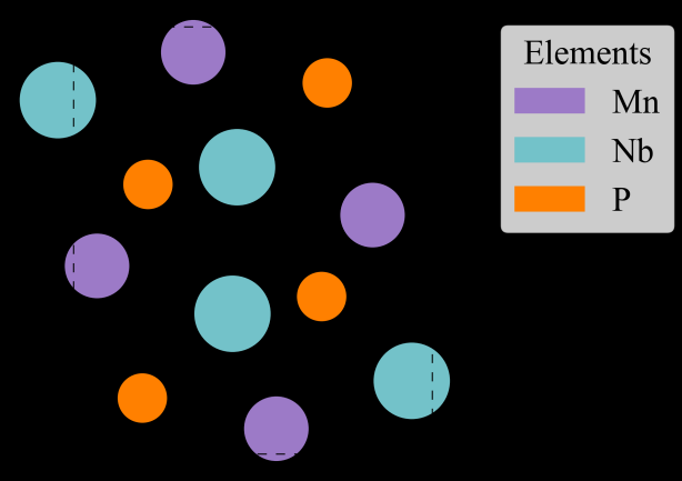
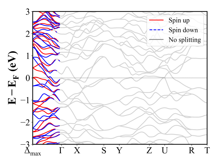
NiPbO3 (R3c) | Band Gap = 0.561 eV
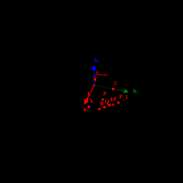
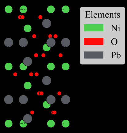
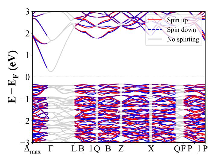
Mn(PbO2)2 (P-42_1c) | Band Gap = 1.458 eV
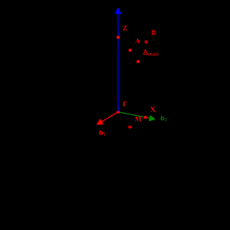
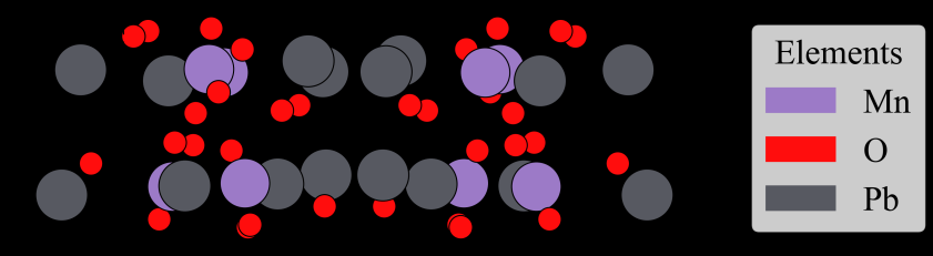
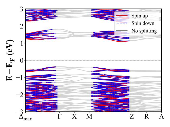
NiCO3 (R-3c) | Band Gap = 4.197 eV
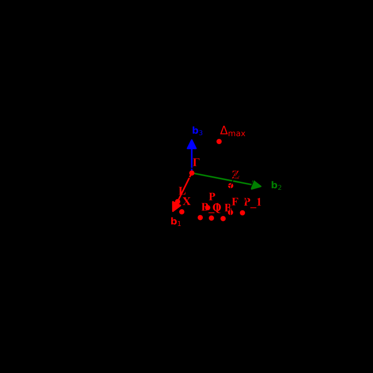
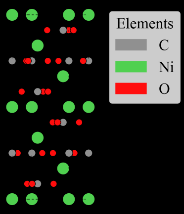
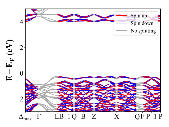
NiTe2O5 (Pnma) | Band Gap = 2.766 eV
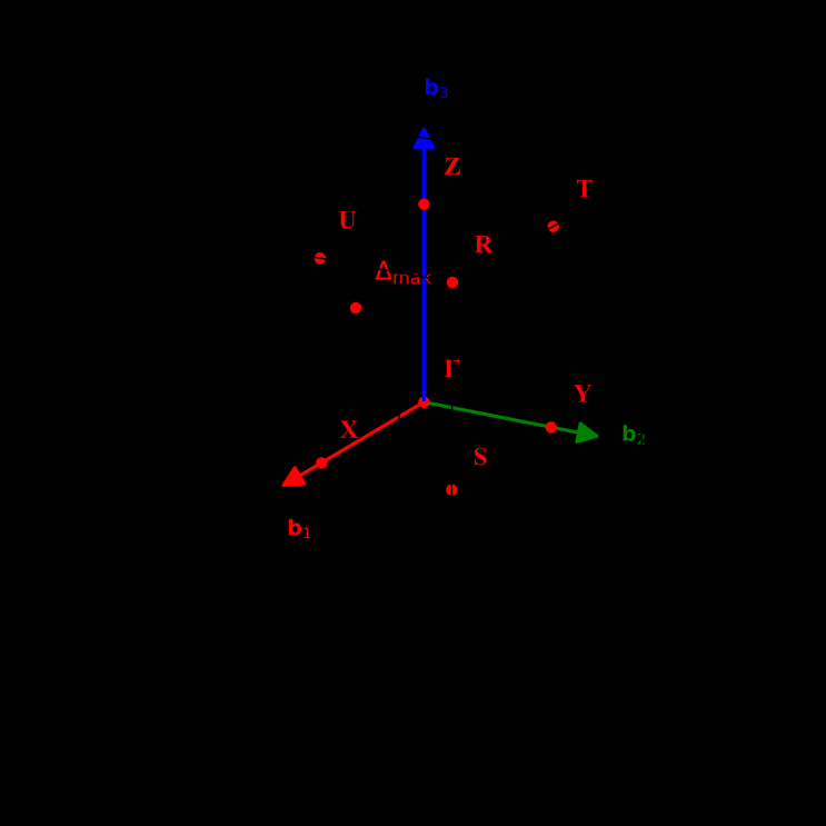
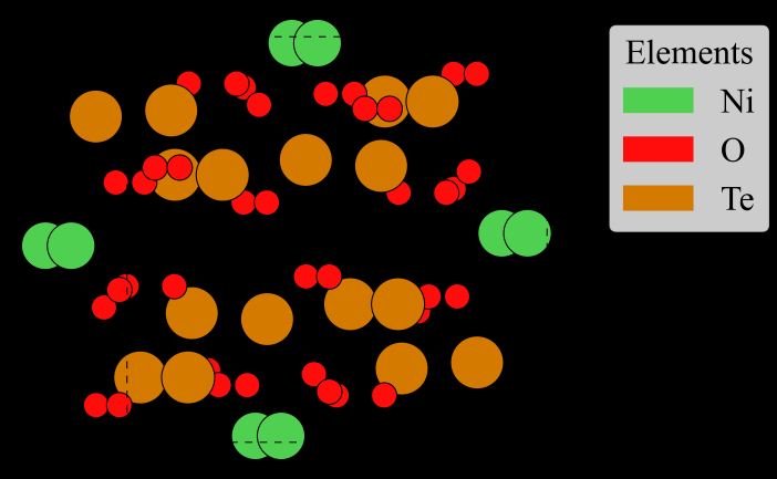
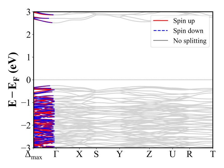
NdVO3 (Pnma) | Band Gap = 1.676 eV
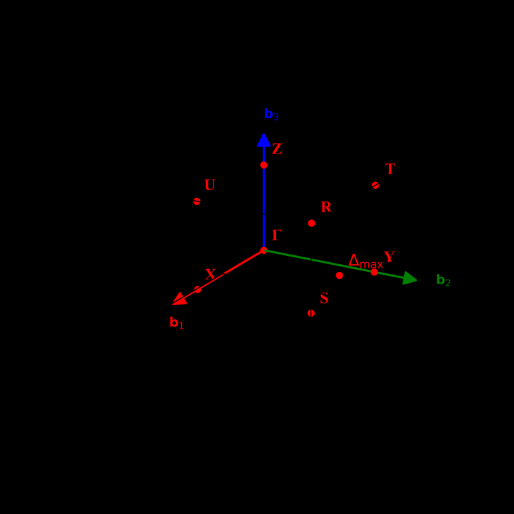
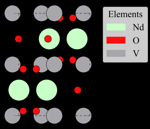
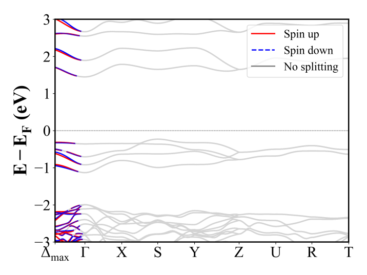
Fe2H4NF6 (Pnma) | Band Gap = 1.828 eV
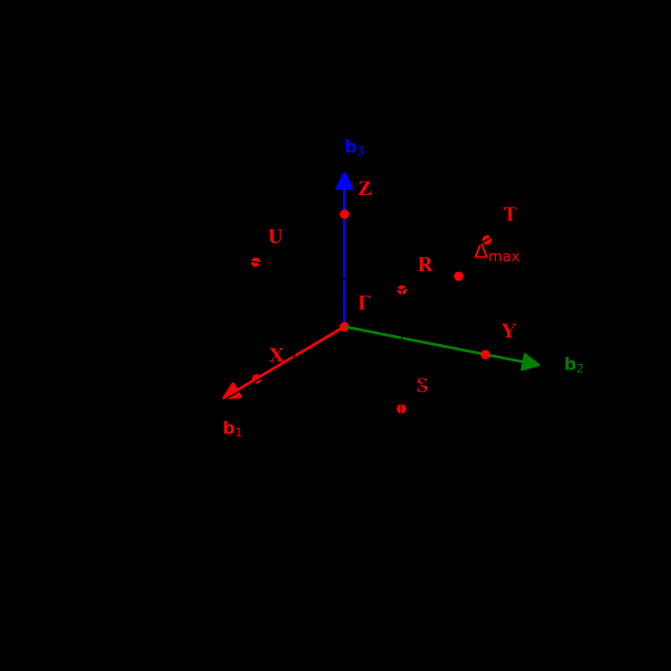
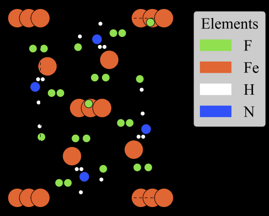
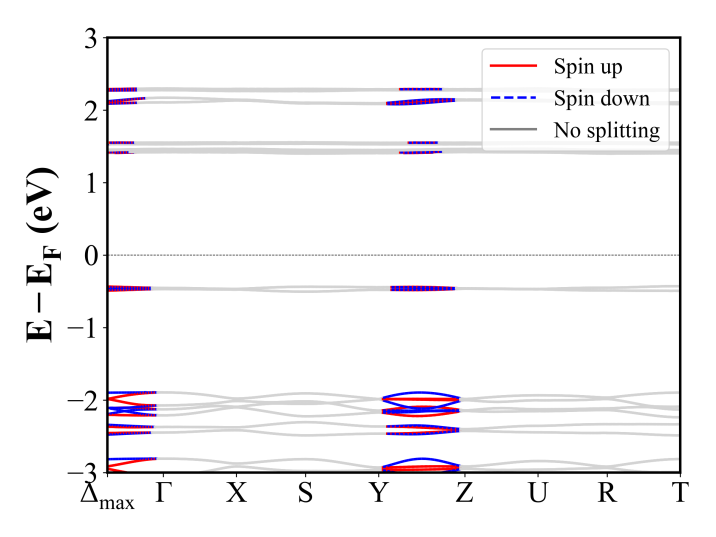
NiF2 (P4_2/mnm) | Band Gap = 5.268 eV
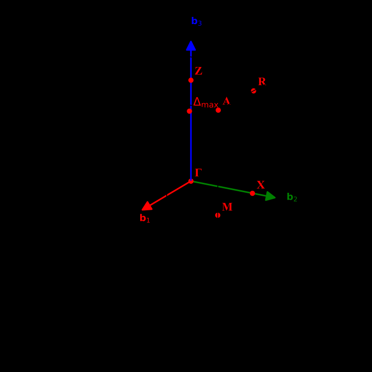
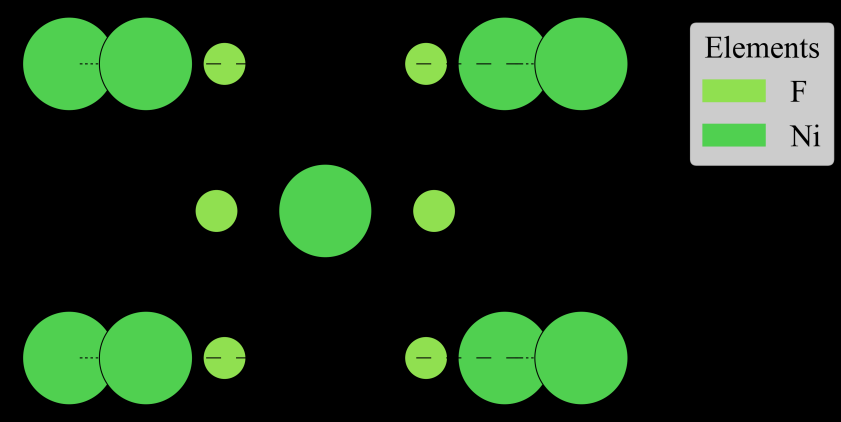
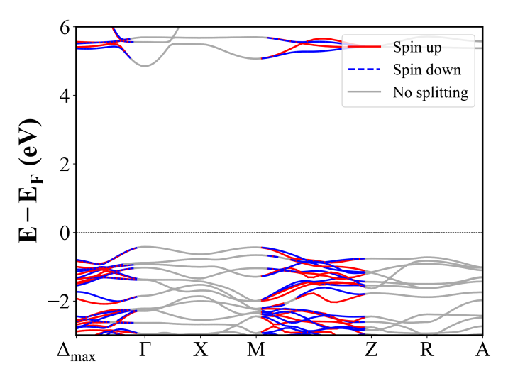
NdMnO3 (Pnma) | Band Gap = 1.420 eV
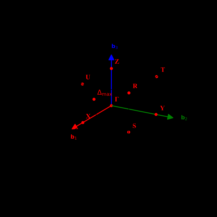
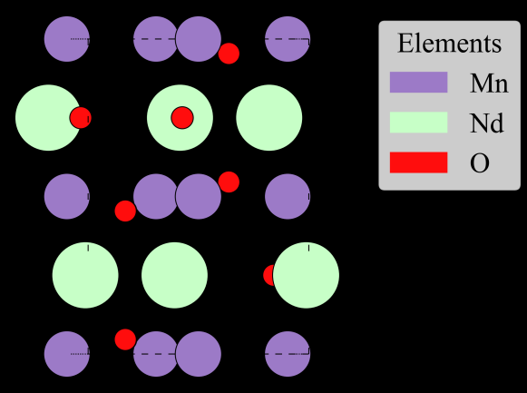
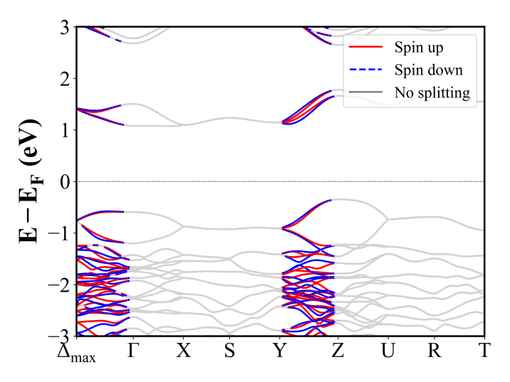
NdFeO3 (Pnma) | Band Gap = 2.833 eV
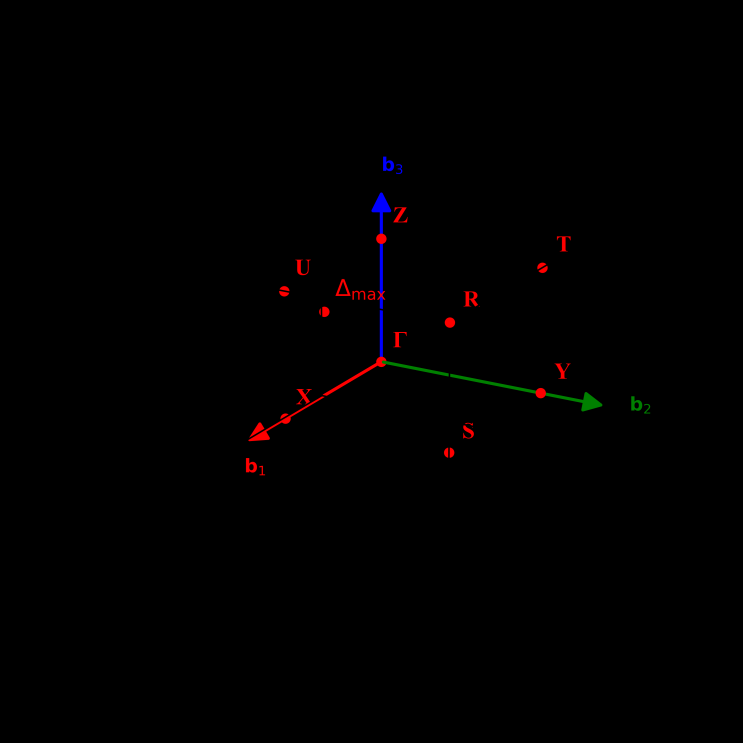
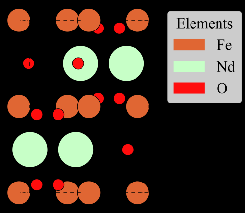
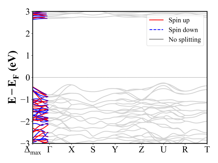
Na2MnH8(C3O5)2 (Pbca)
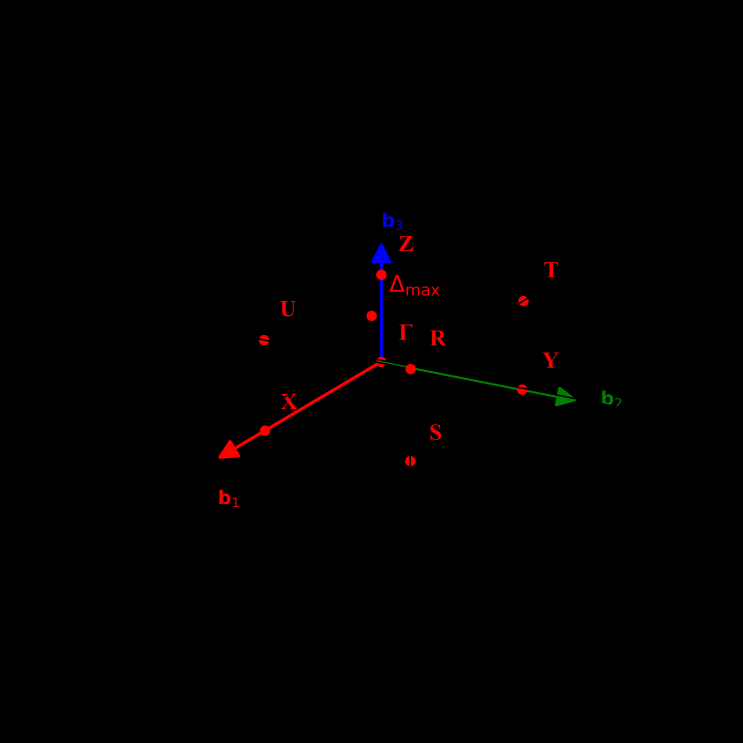
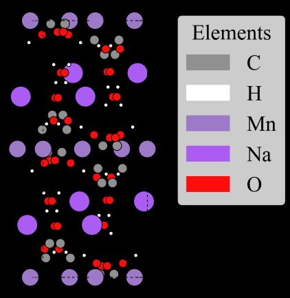
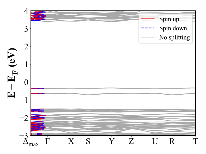
BaNa2V2FeO8 (C2/c) | Band Gap = 2.710 eV
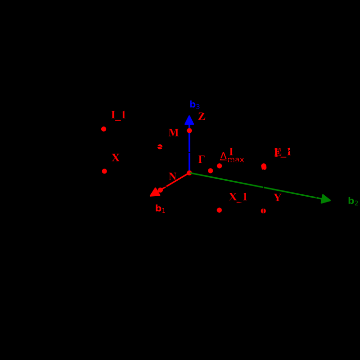
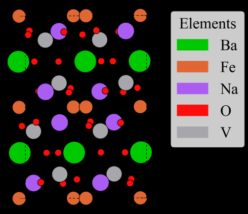
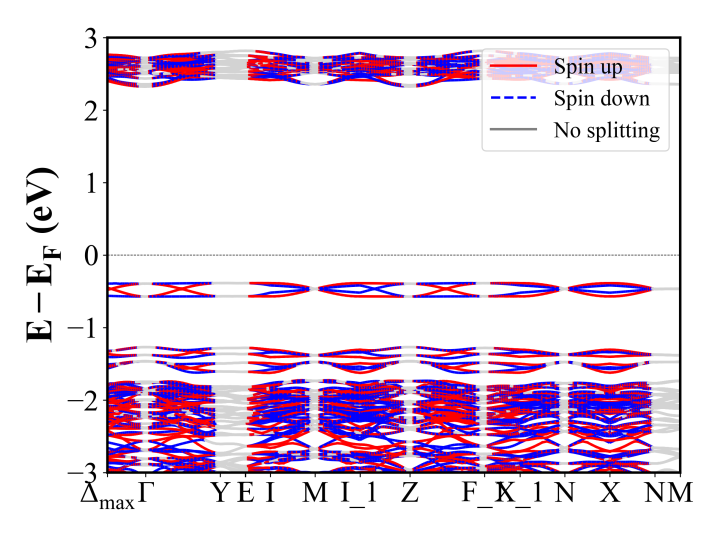
CrNiO4 (Cmcm) | Band Gap = 2.000 eV
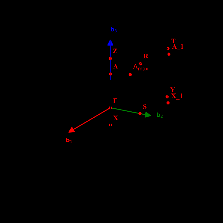
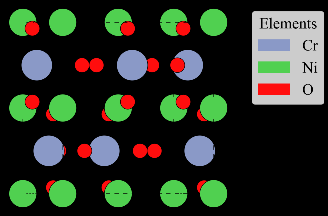
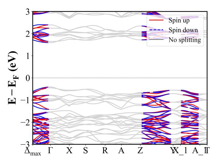
NdCrO3 (Pnma) | Band Gap = 3.079 eV
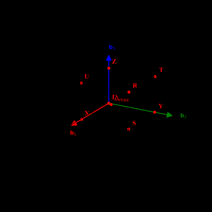
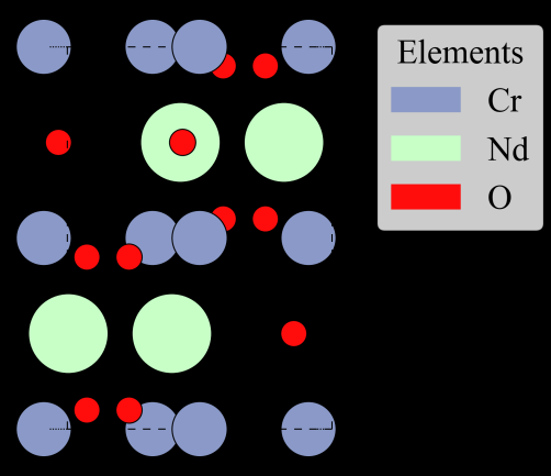
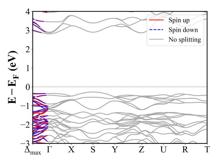
FeNiPO5 (Pnma) | Band Gap = 2.694 eV
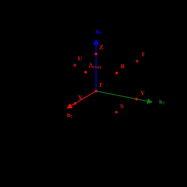
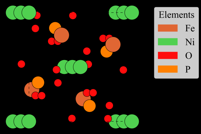
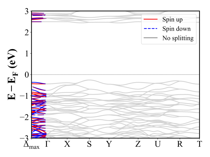
Sr2CoTeO6 (P2_1/c) | Band Gap = 2.154 eV
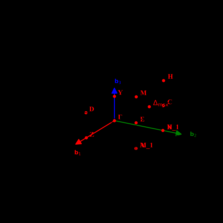
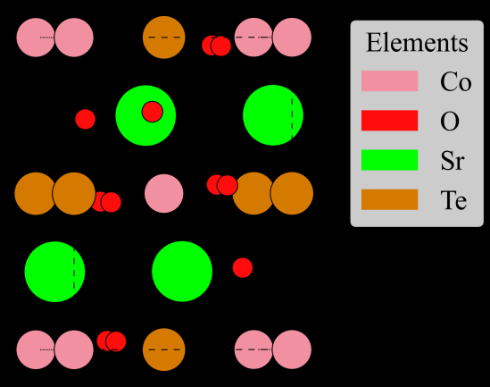
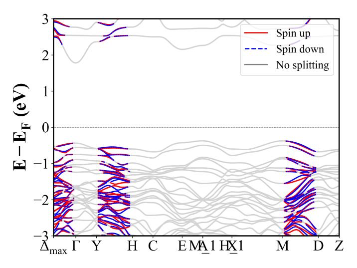
Sr2ScOsO6 (P2_1/c) | Band Gap = 0.000 eV
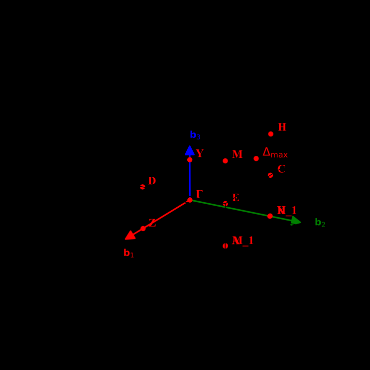
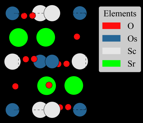
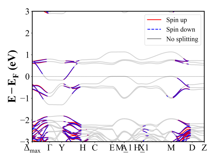
PrFeO3 (Pnma) | Band Gap = 2.822 eV
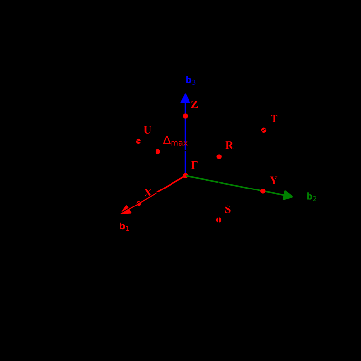
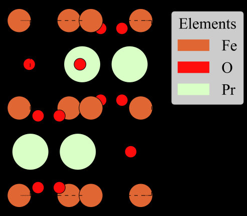
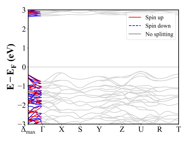
Sr2ErRuO6 (P2_1/c) | Band Gap = 1.009 eV
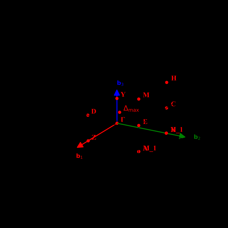
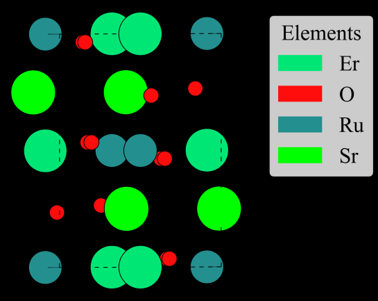
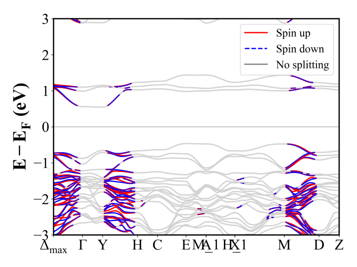
Sr2MnTeO6 (P2_1/c) | Band Gap = 1.792 eV
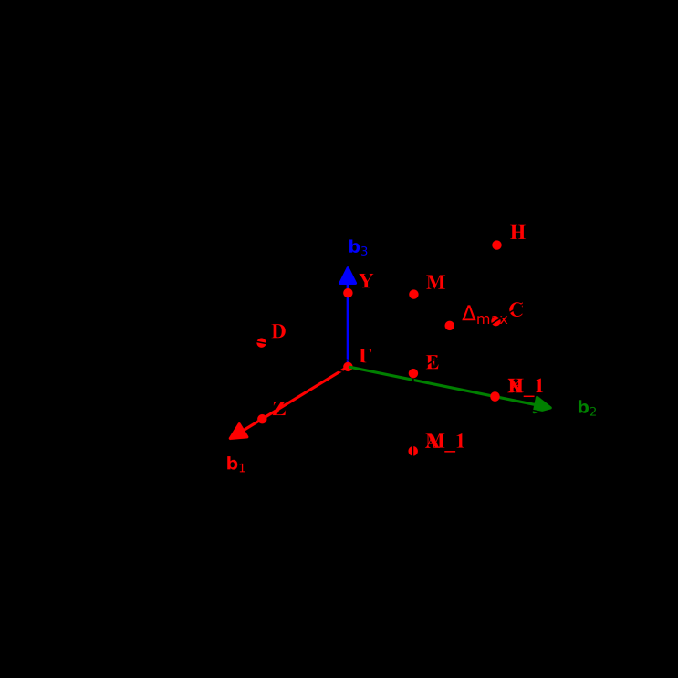
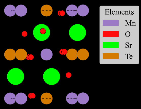
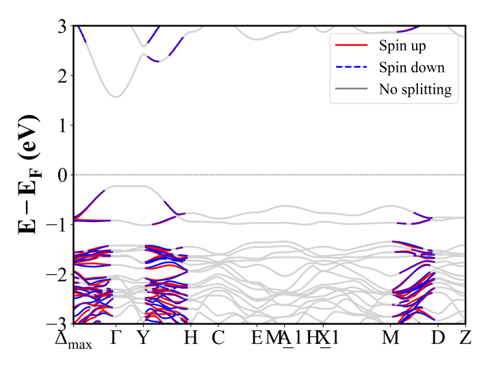
PrMnO3 (Pnma) | Band Gap = 0.892 eV
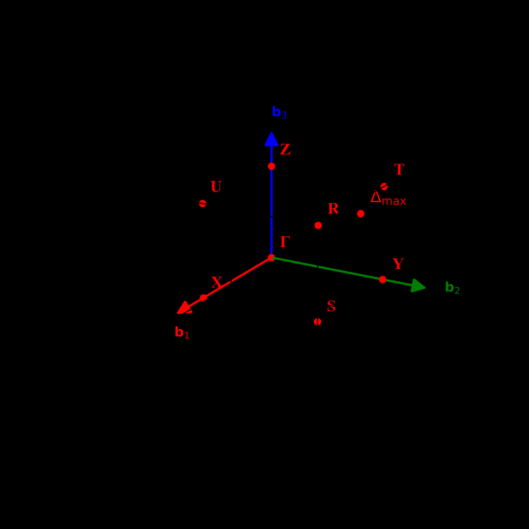
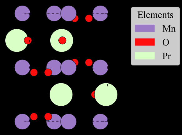
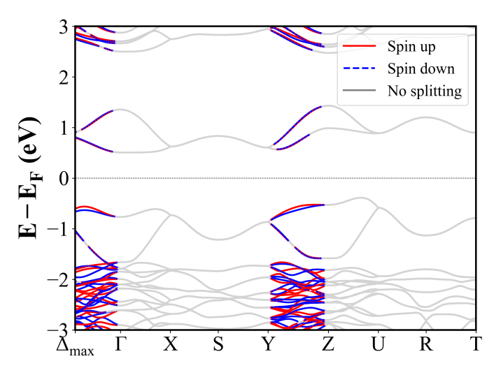
Sr2CoOsO6 (C2/c) | Band Gap = 0.000 eV
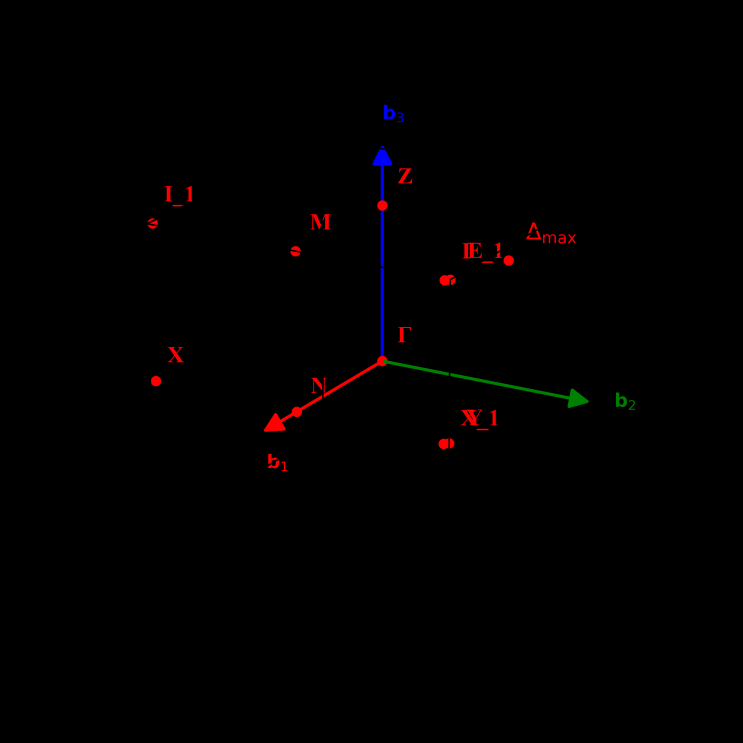
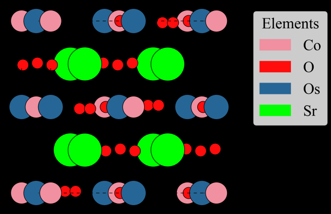
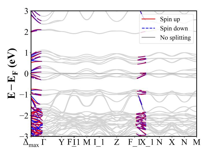
RbFe2F6 (Pnma) | Band Gap = 1.744 eV
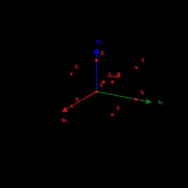
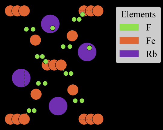
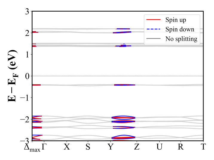
BaPrMn2O6 (Pmc2_1) | Band Gap = 0.000 eV
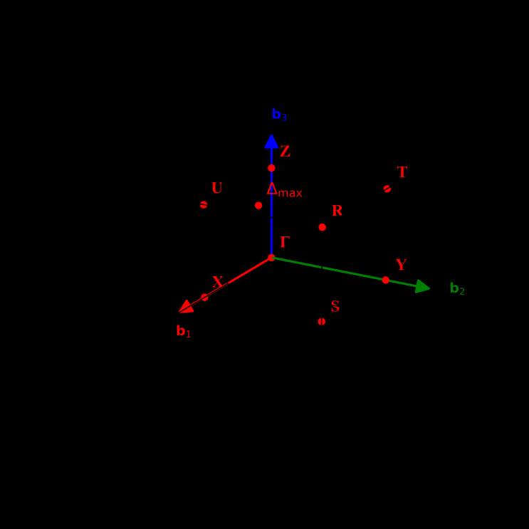
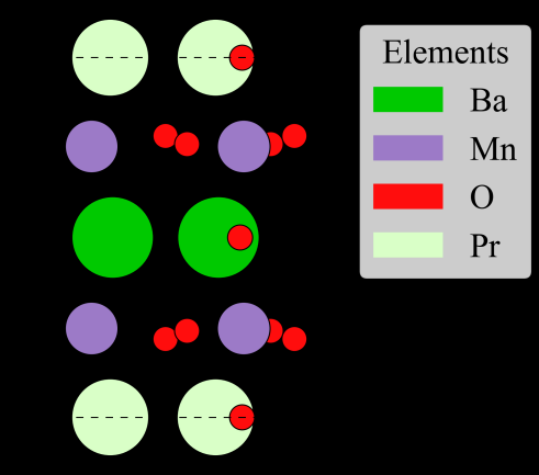
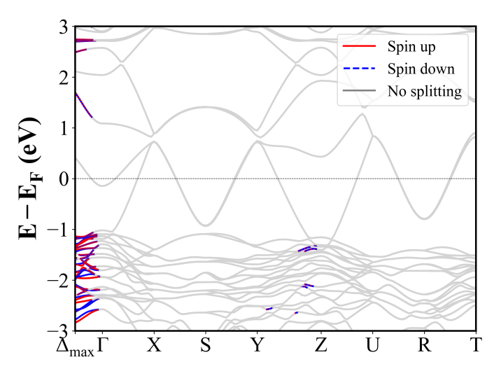
Sr2NiTeO6 (P2_1/c) | Band Gap = 2.343 eV
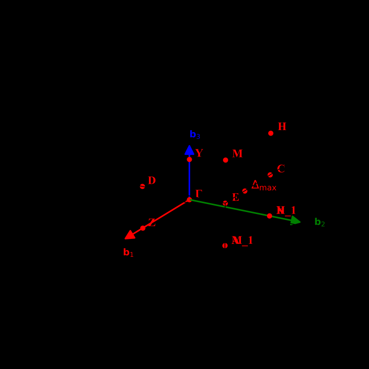
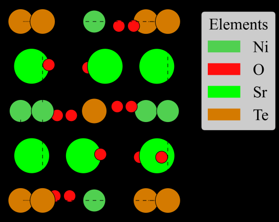
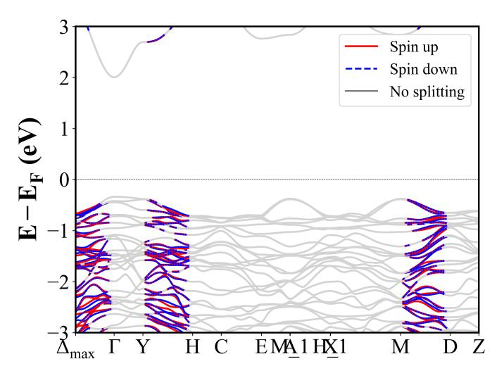
RbMnF4 (P2_1/c) | Band Gap = 1.926 eV
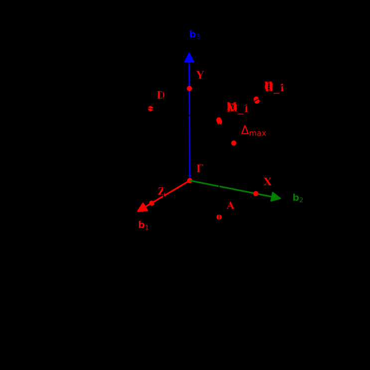
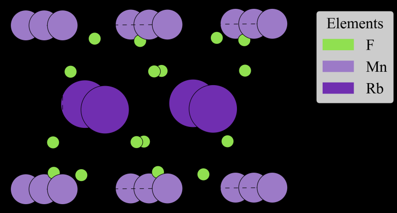
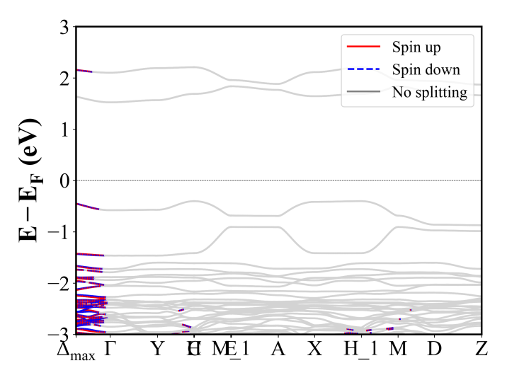
RbCoBr3 (P6_3/mmc) | Band Gap = 0.000 eV
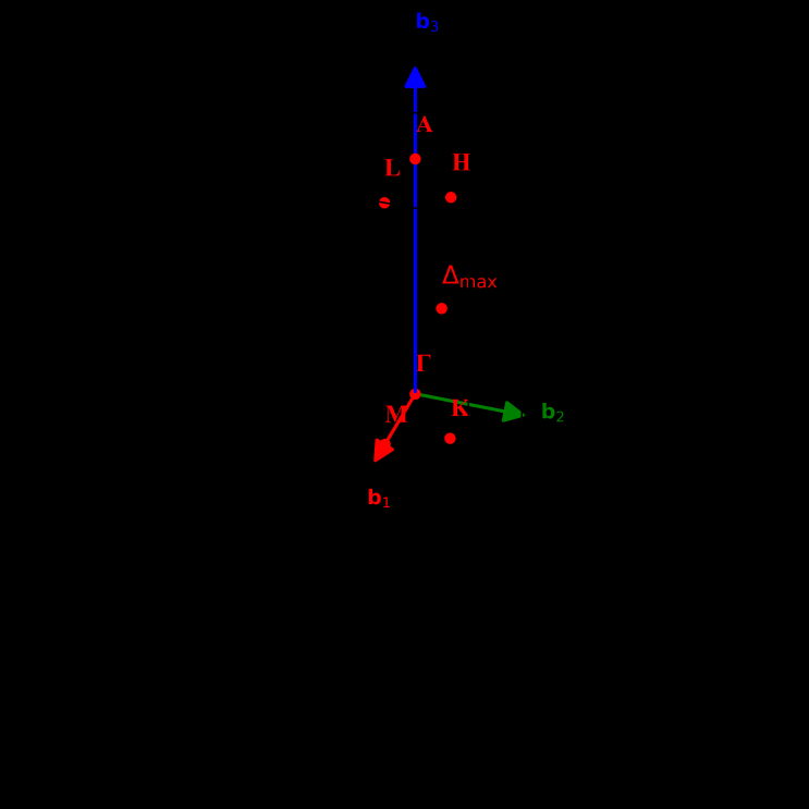
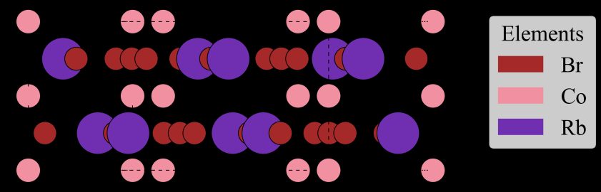
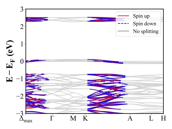
Sr2HoRuO6 (P2_1/c) | Band Gap = 1.031 eV
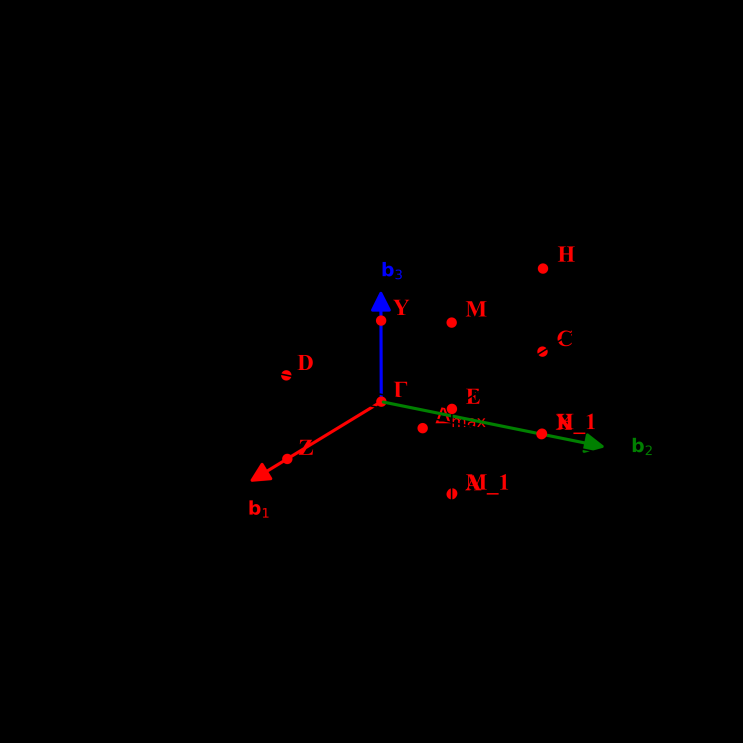
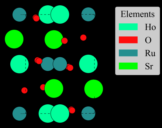
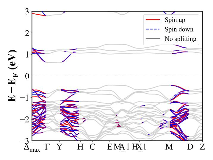
Sr2LuRuO6 (P2_1/c) | Band Gap = 0.958 eV
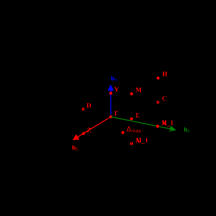
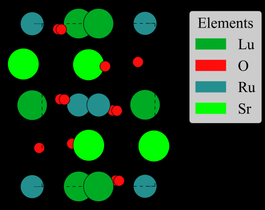
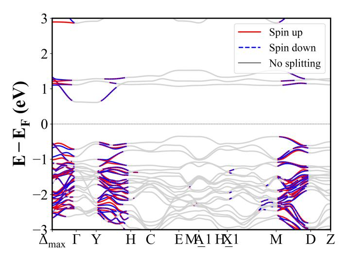
Sr2DyRuO6 (P2_1/c) | Band Gap = 1.114 eV
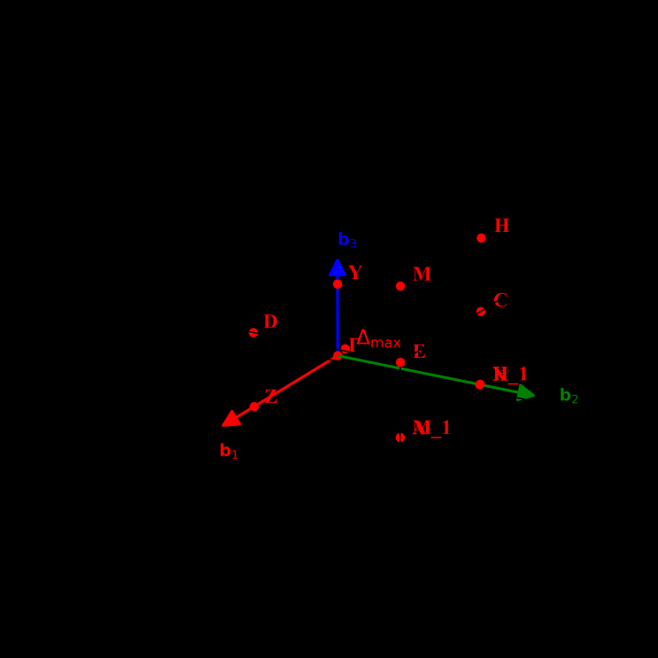
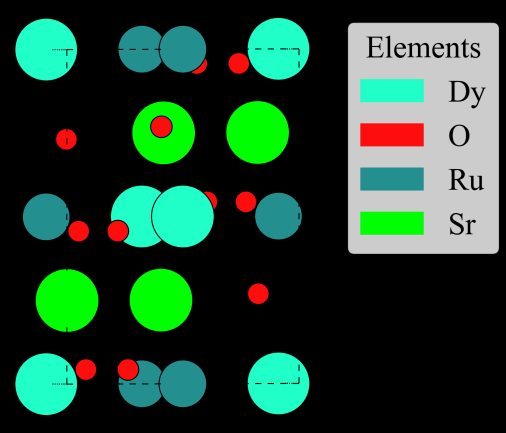
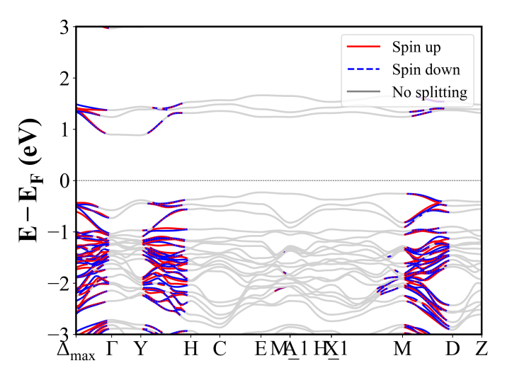
SmCrO3 (Pnma) | Band Gap = 3.106 eV
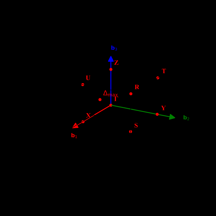
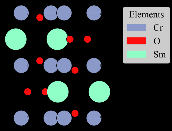
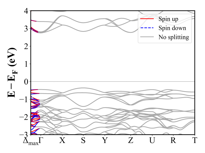
ScMnO3 (P6_3cm) | Band Gap = 1.400 eV
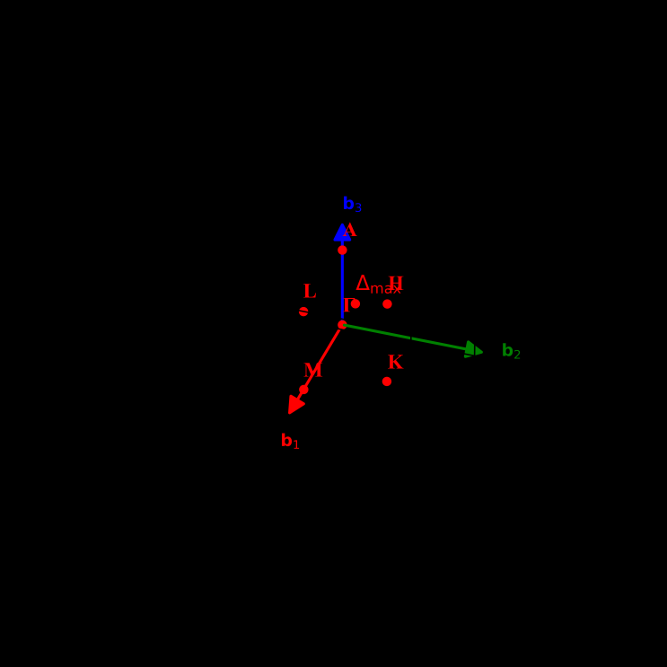
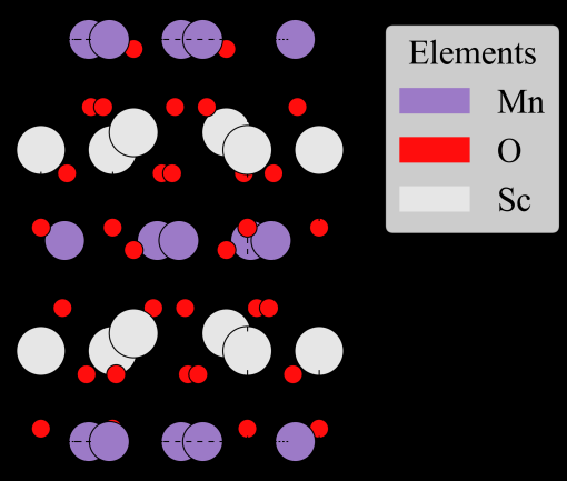
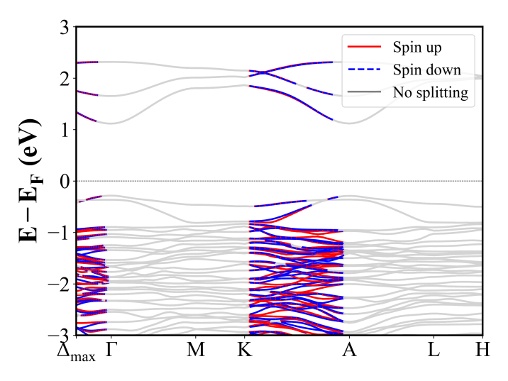
ScCrO3 (Pnma) | Band Gap = 2.987 eV
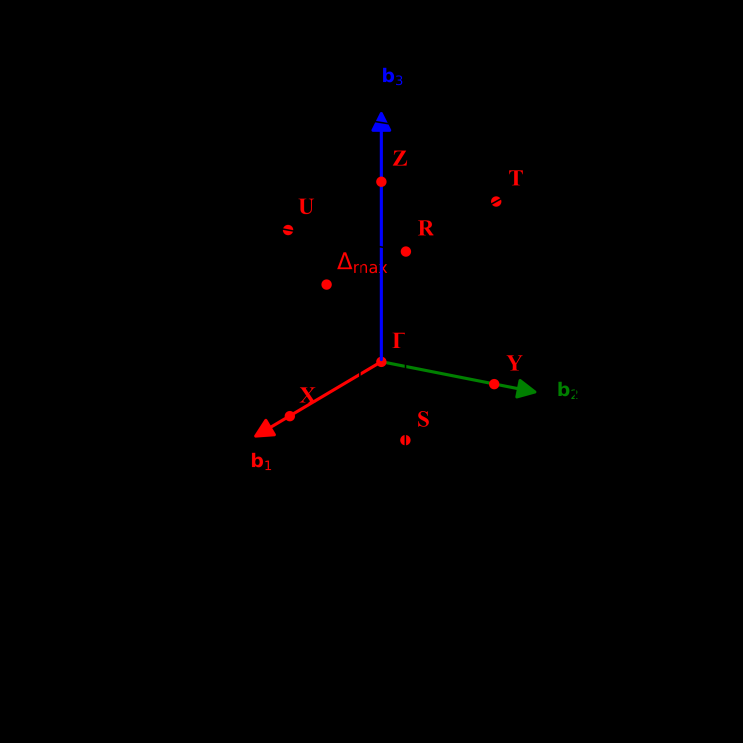
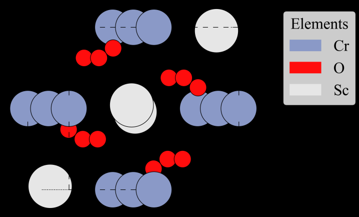
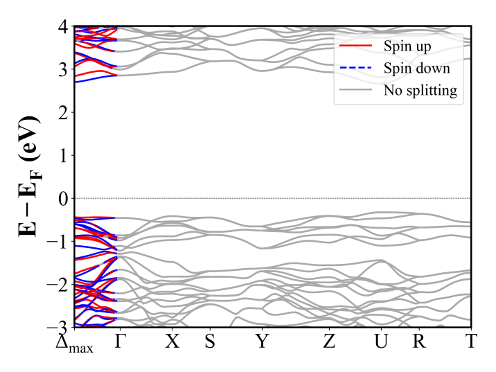
RuO2 (P4_2/mnm) | Band Gap = 0.000 eV
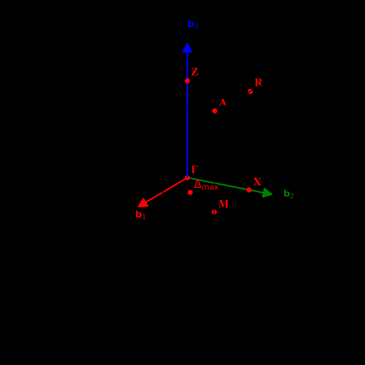
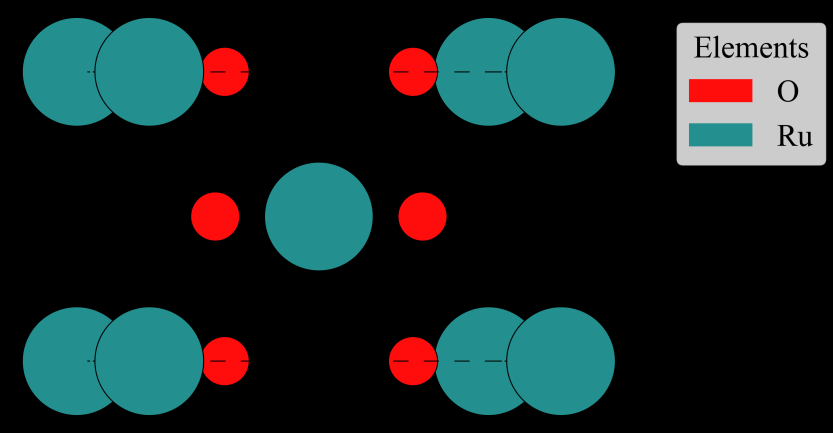
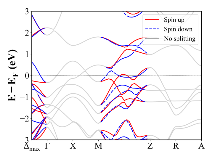
SmFeO3 (Pnma) | Band Gap = 2.843 eV
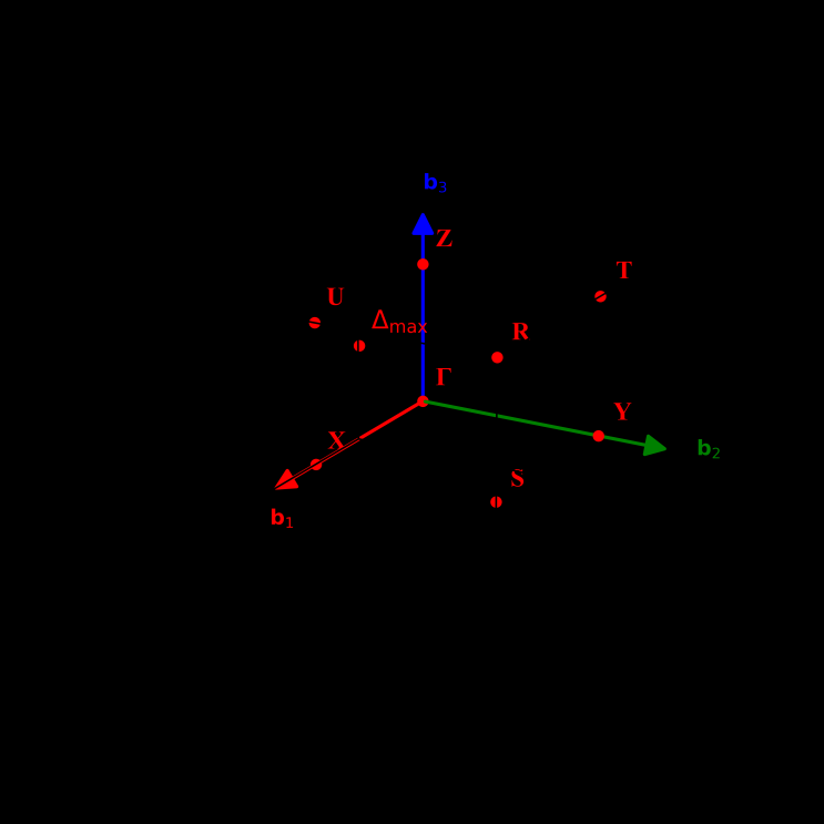
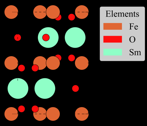
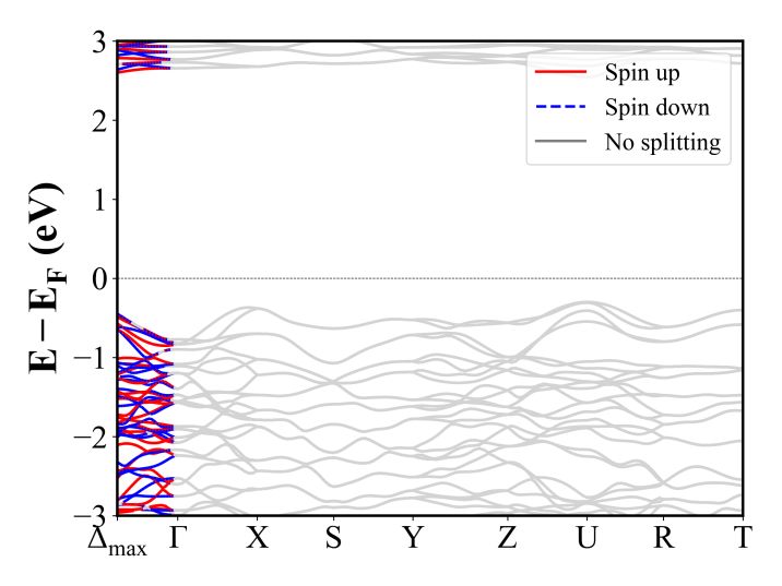
Sr2TbRuO6 (P2_1/c) | Band Gap = 1.044 eV
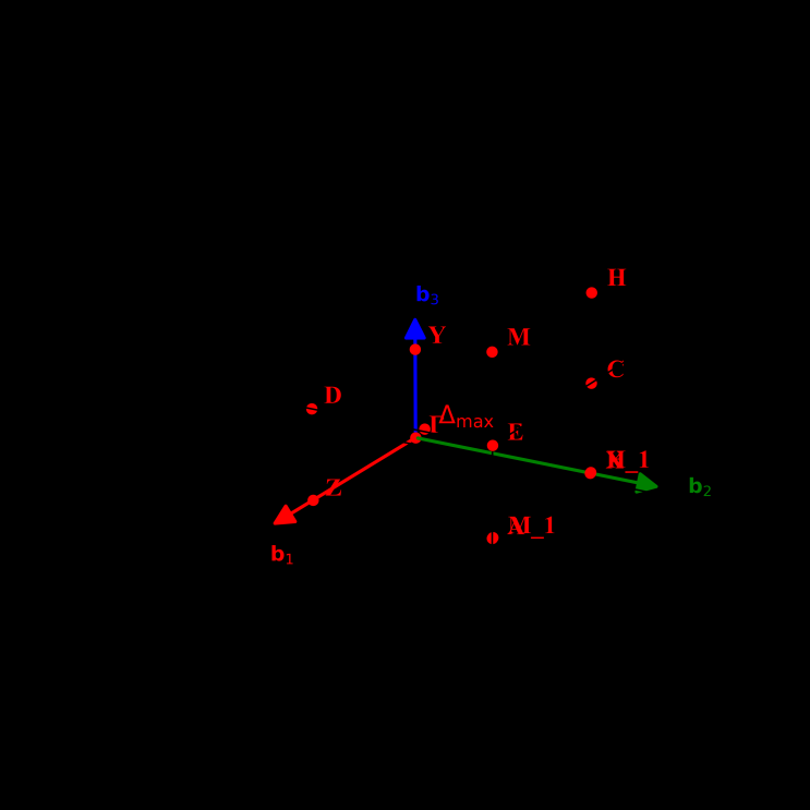
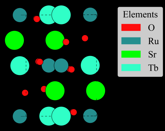
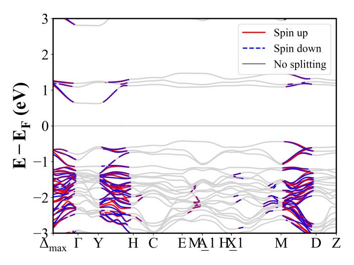
SrMnVHO5 (P2_12_12_1) | Band Gap = 2.356 eV
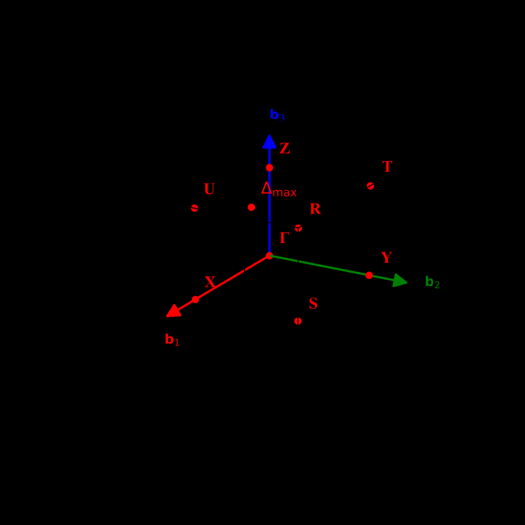
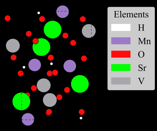
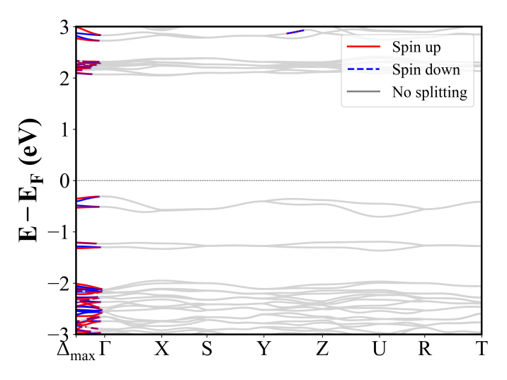
Sr2TmRuO6 (P2_1/c) | Band Gap = 0.978 eV
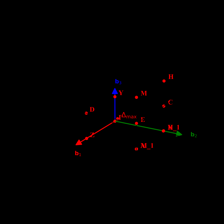
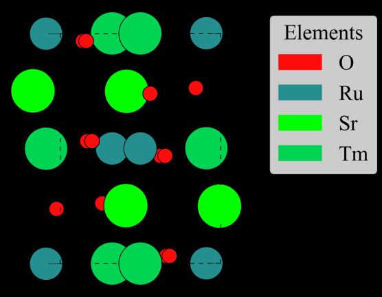
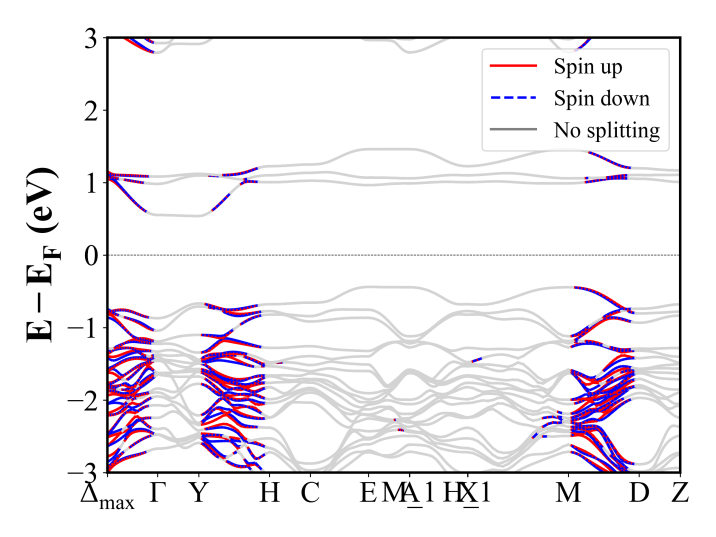
NaSr3RuO6 (R-3c) | Band Gap = 1.568 eV
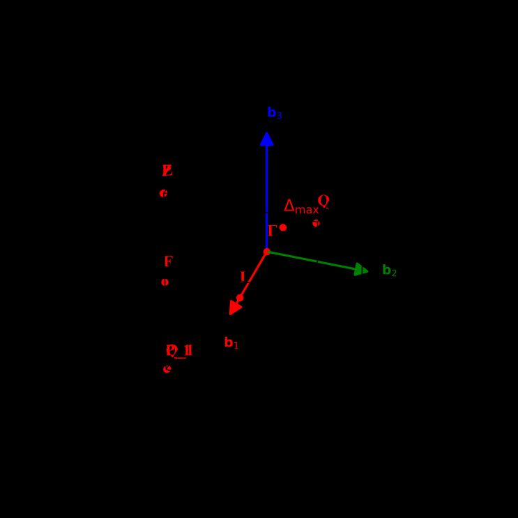
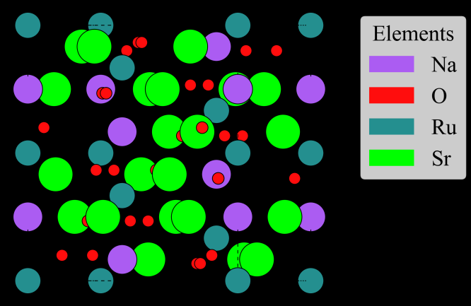
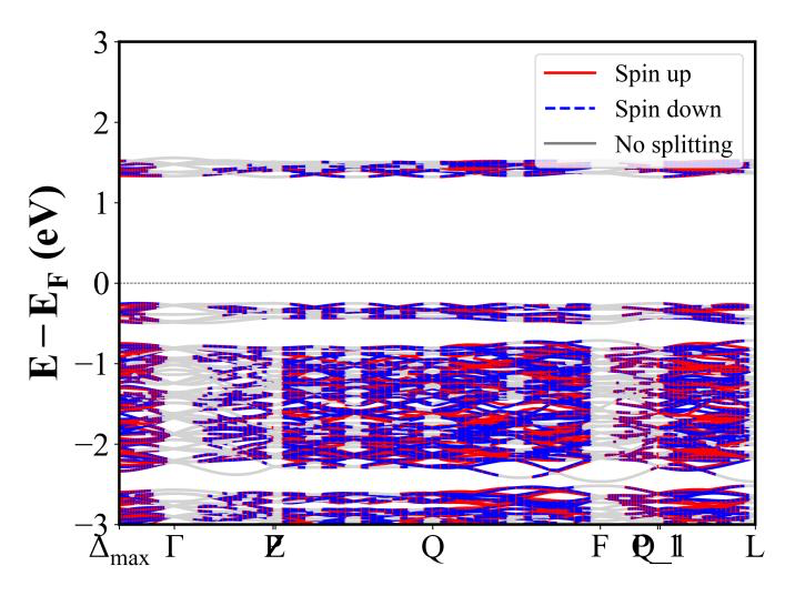
TbCrO3 (Pnma) | Band Gap = 3.114 eV
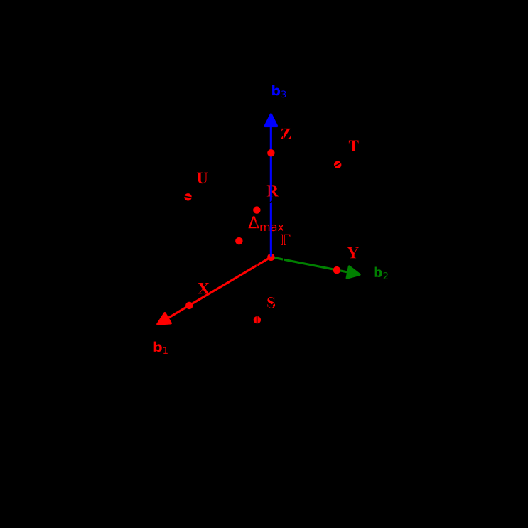
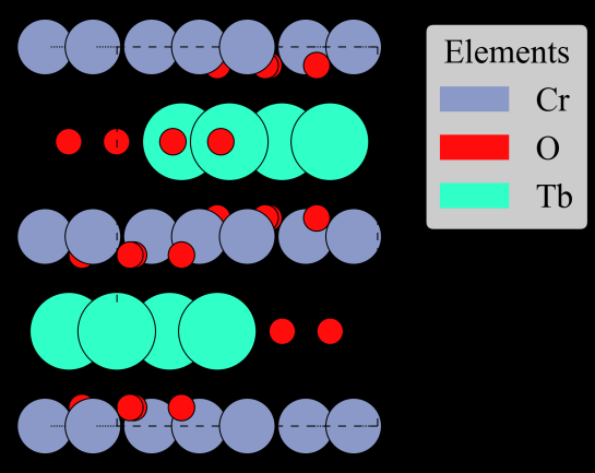
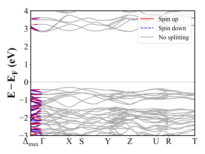
SrMnO3 (C222_1) | Band Gap = 1.873 eV
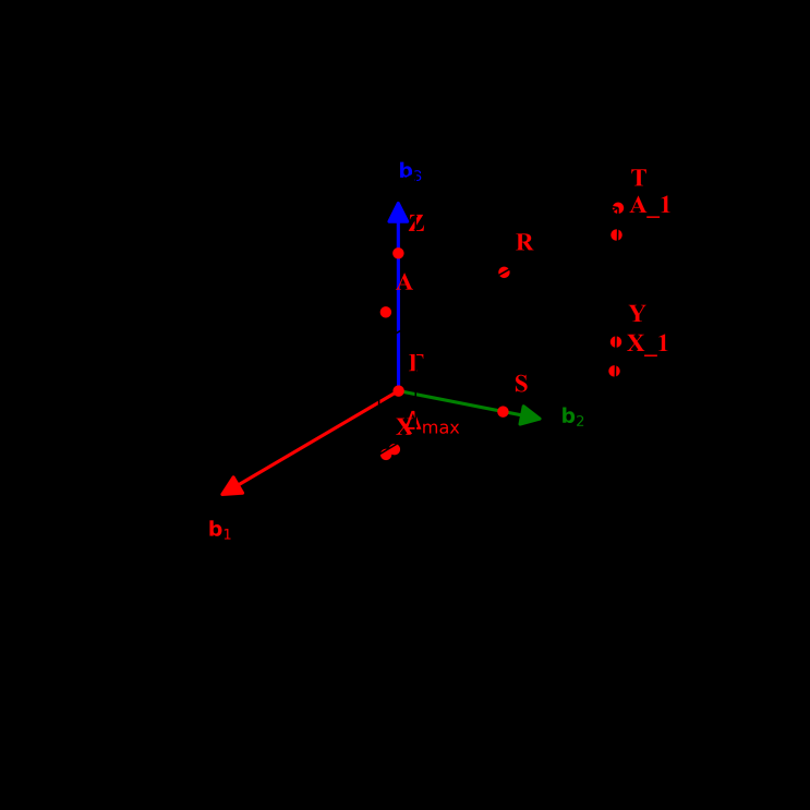
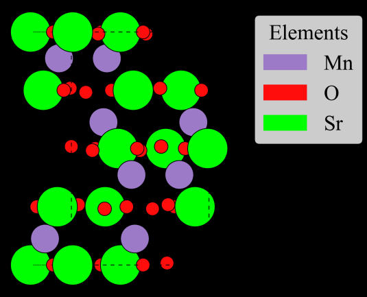
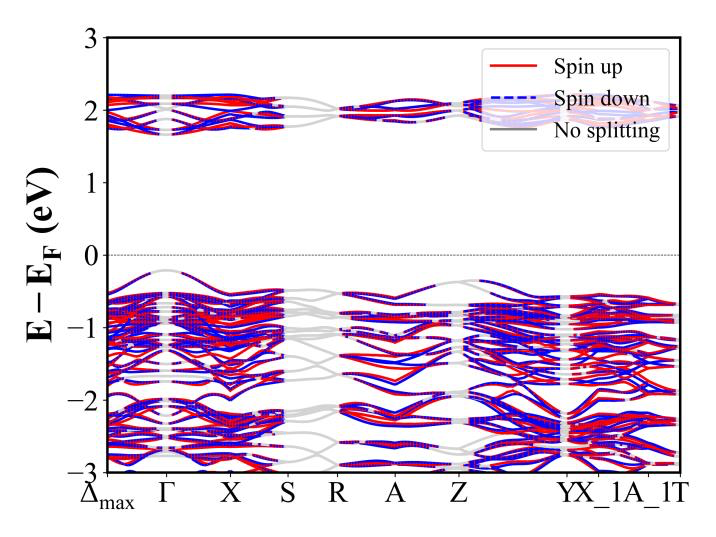
Sr2YRuO6 (P2_1/c) | Band Gap = 1.012 eV
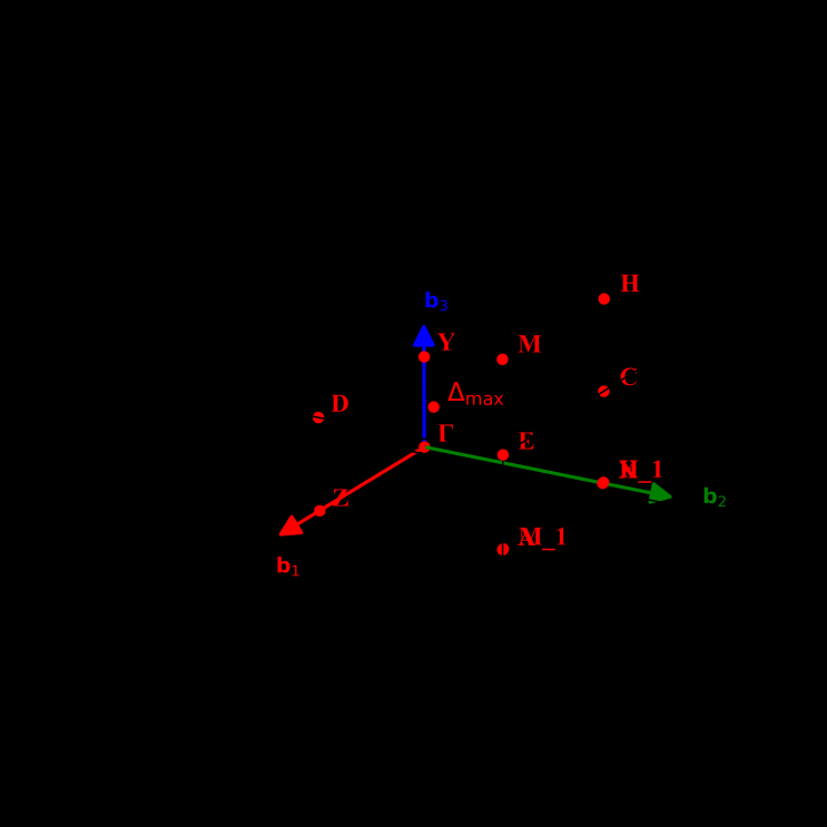
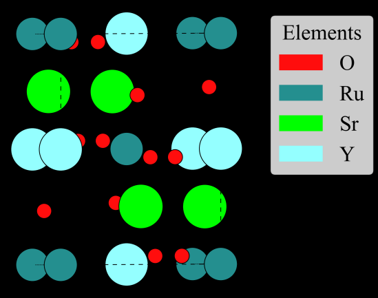
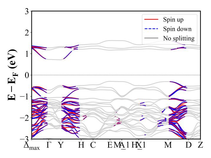
TbFeO3 (Pnma) | Band Gap = 2.826 eV
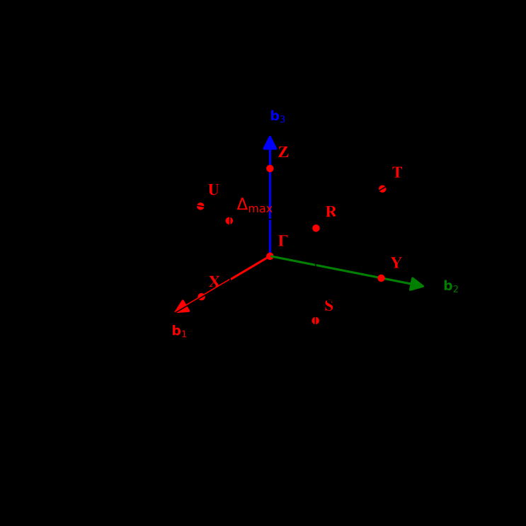
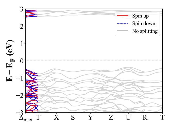
TmCrO3 (Pnma) | Band Gap = 3.141 eV
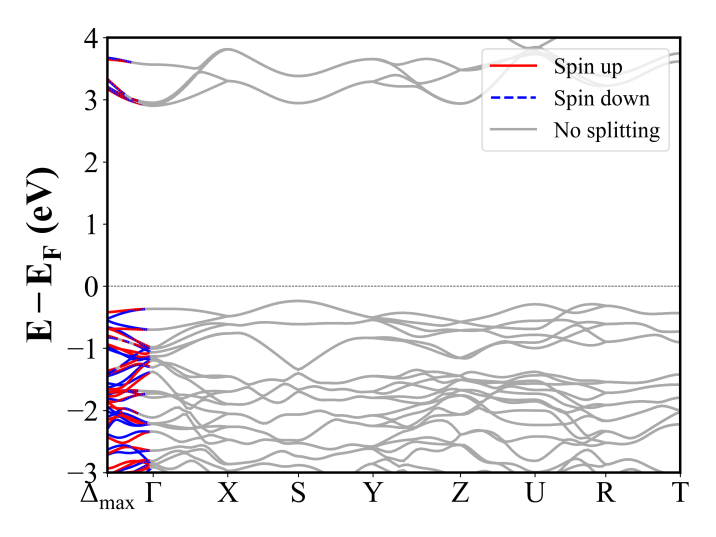
TmFeO3 (Pnma) | Band Gap = 0.745 eV
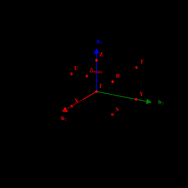
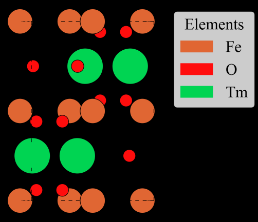
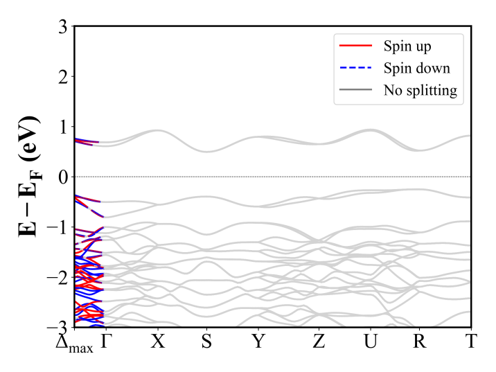
TmVO3 (Pnma) | Band Gap = 2.050 eV
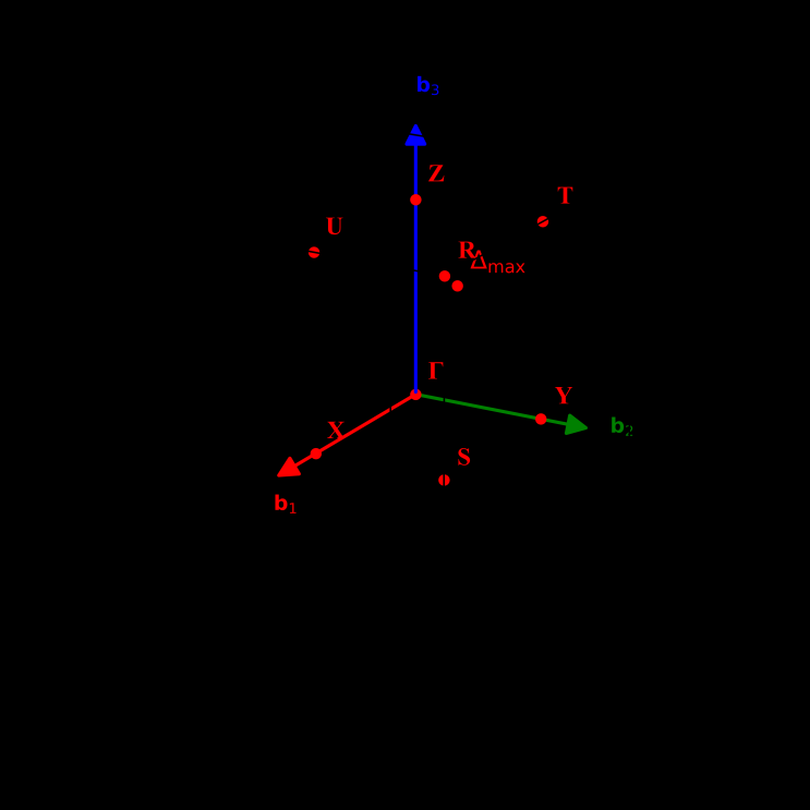
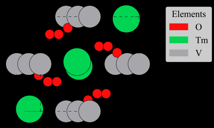
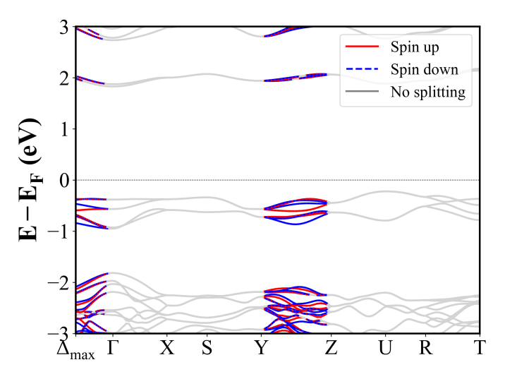
Sr4Fe4O11 (Cmmm) | Band Gap = 0.176 eV
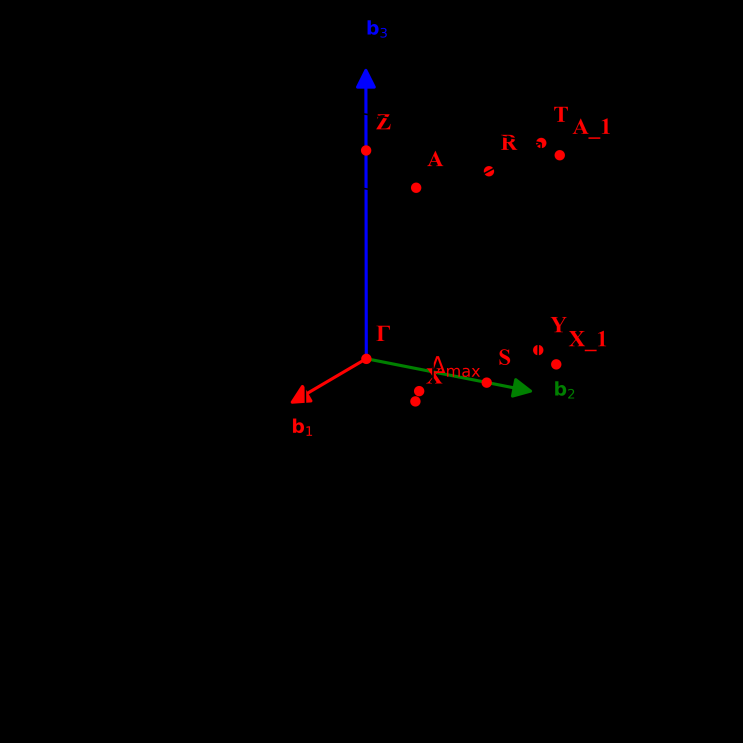
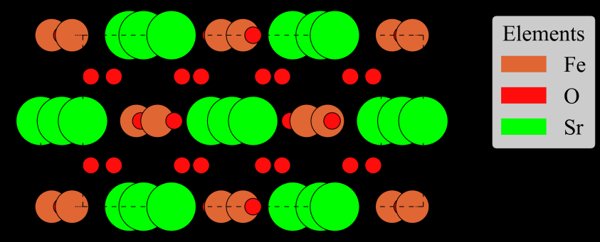
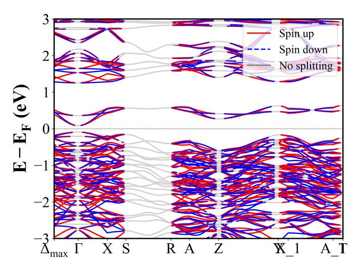
Sr2YbRuO6 (P2_1/c) | Band Gap = 0.981 eV
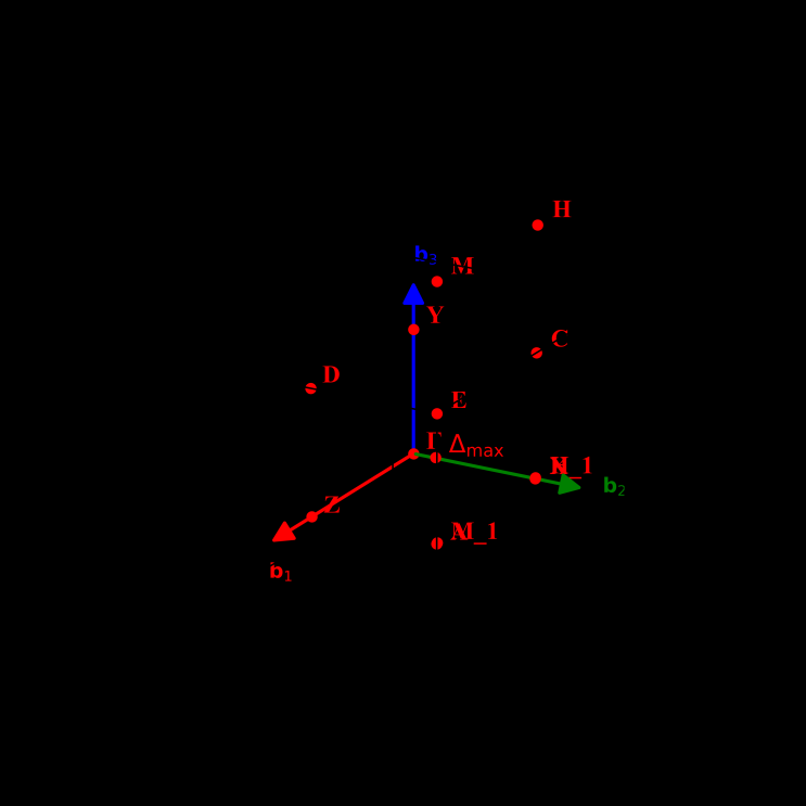
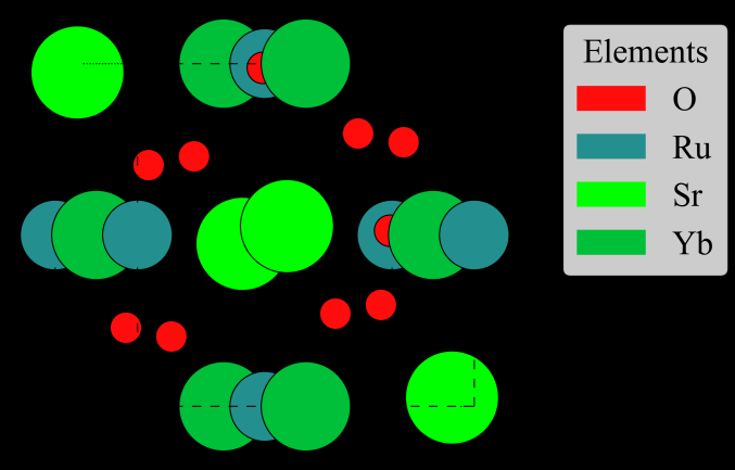
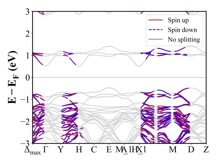
Sr2TbIrO6 (P2_1/c) | Band Gap = 0.139 eV
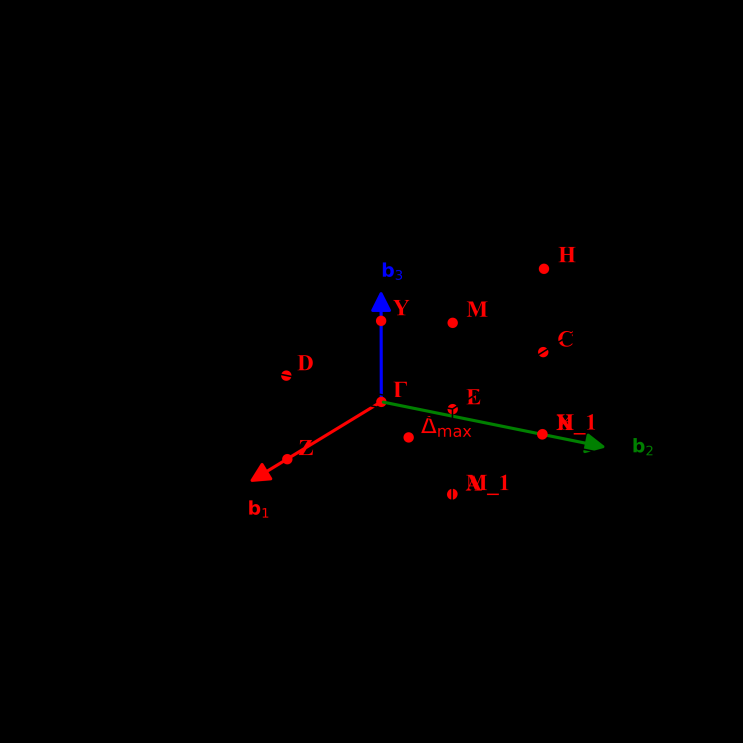
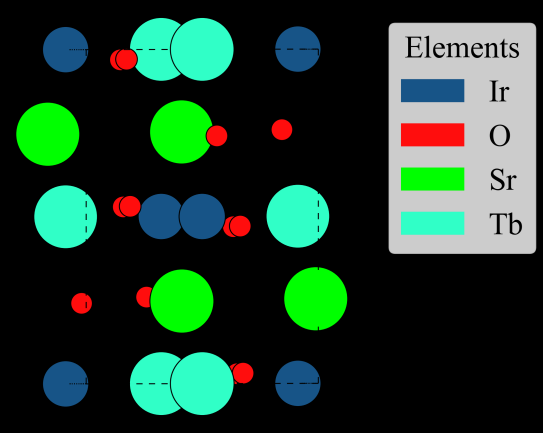
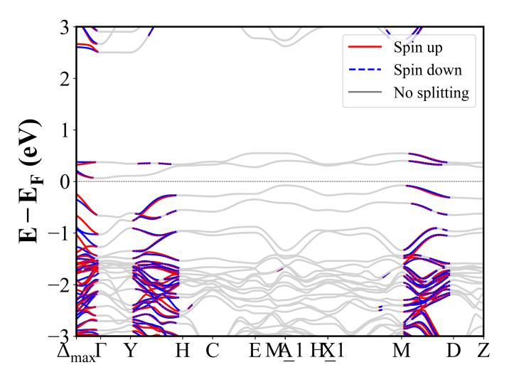
TlCrO3 (Pnma) | Band Gap = 0.625 eV
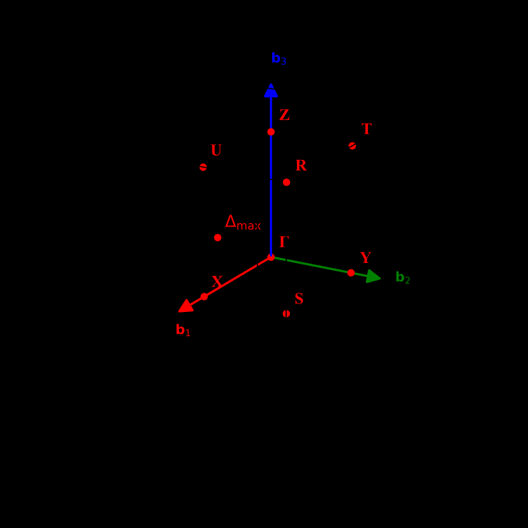
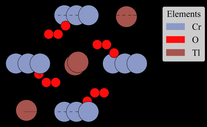
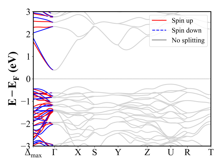
Sr3LiRuO6 (R-3c) | Band Gap = 1.553 eV
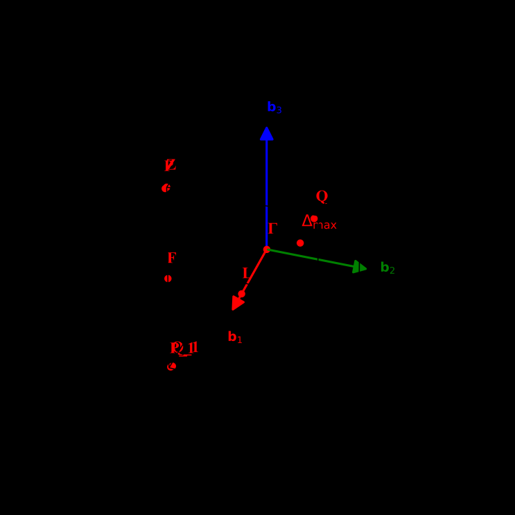
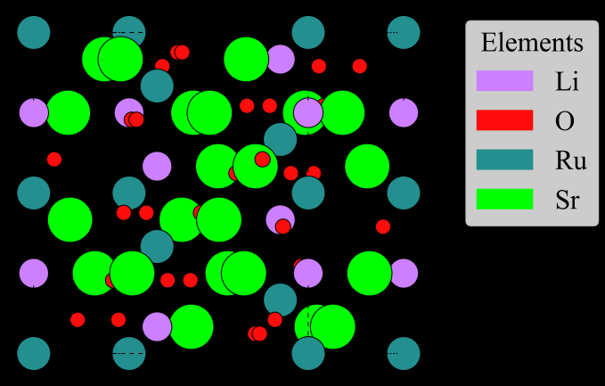
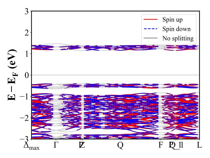
SrMn2V2O8 (I4_1cd) | Band Gap = 2.760 eV
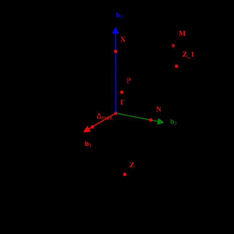
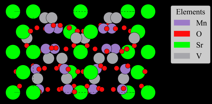
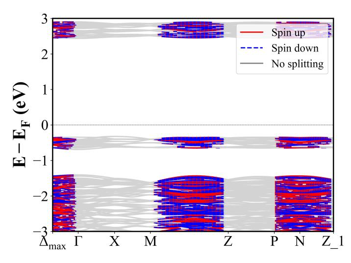
YMnO3 (P6_3cm) | Band Gap = 1.304 eV
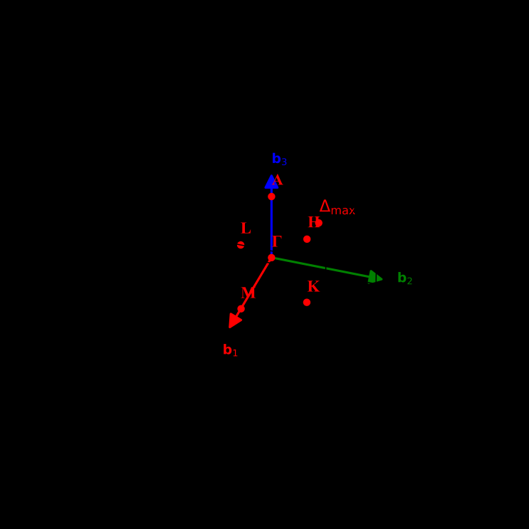
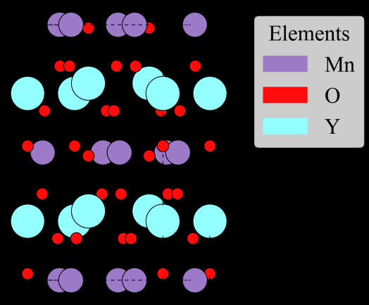
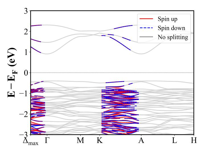
Nb3VS6 (P6_322) | Band Gap = 0.000 eV
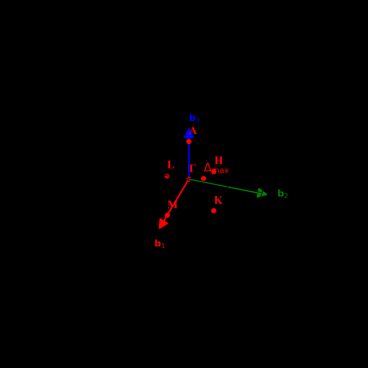
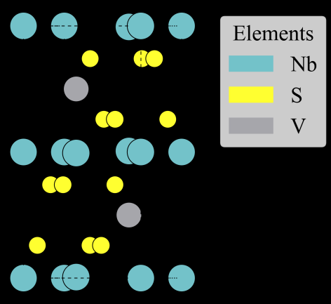
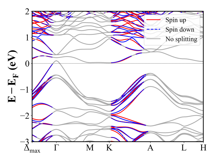
YVO3 (P2_1/c) | Band Gap = 2.012 eV
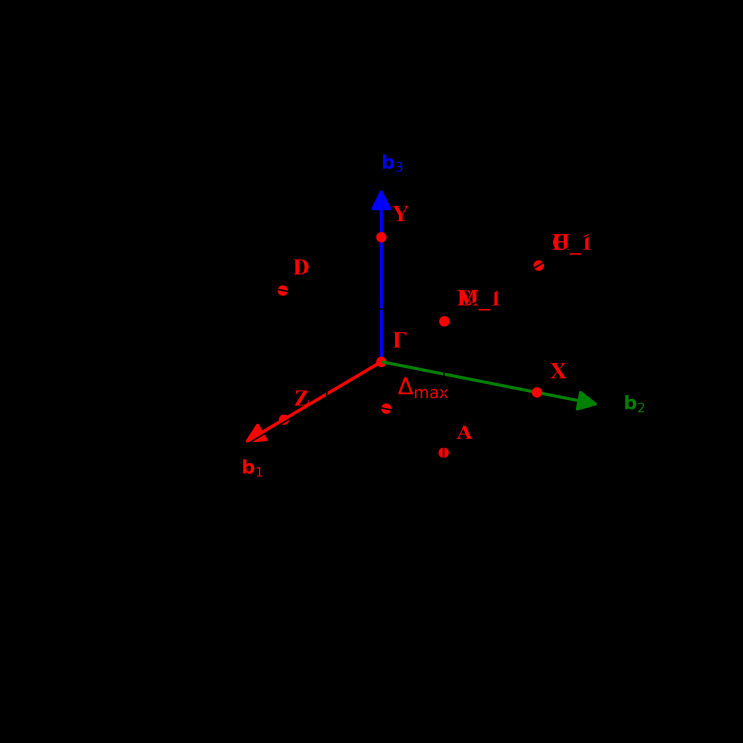
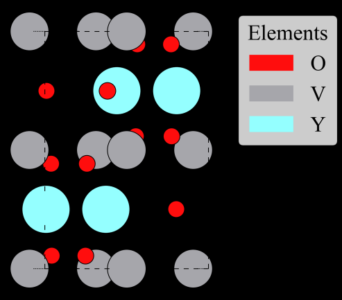
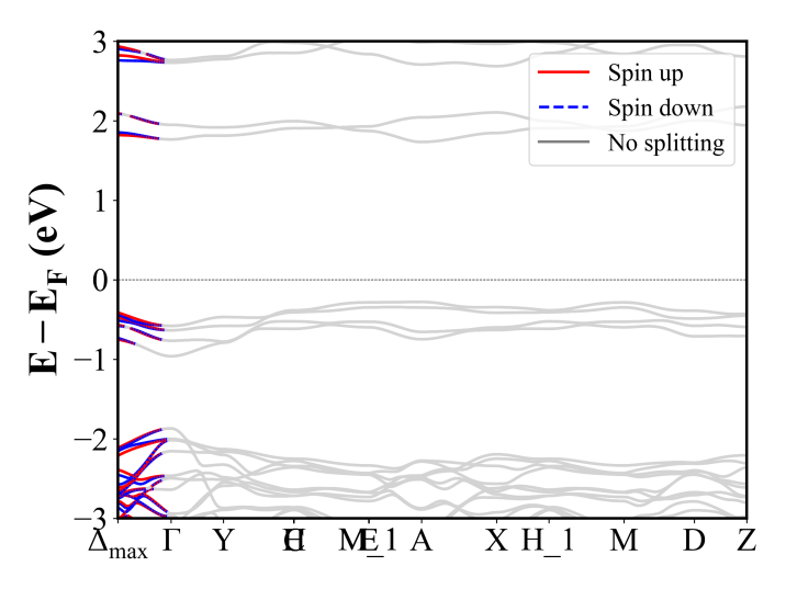
TmVO3 (P2_1/c) | Band Gap = 1.739 eV
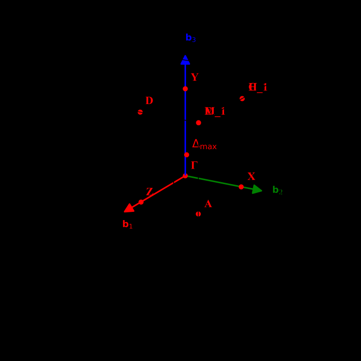
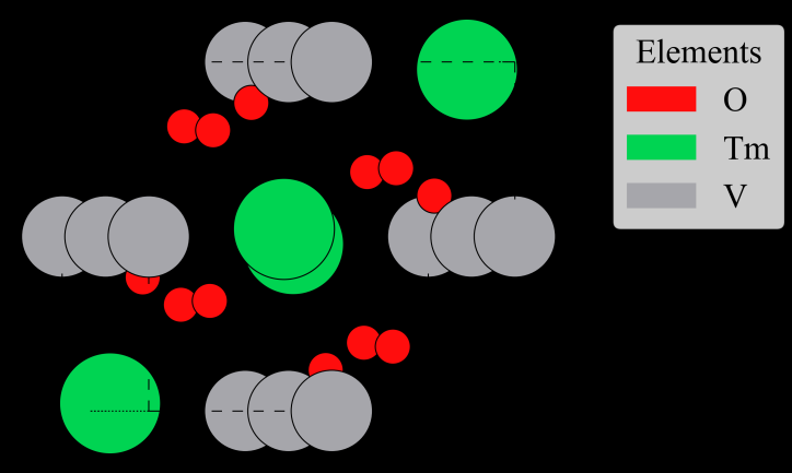
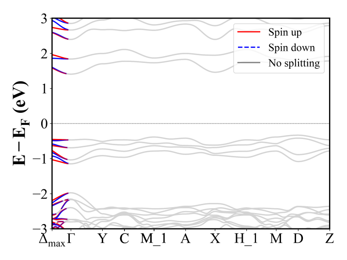
Y2Cu2O5 (Pna2_1) | Band Gap = 1.704 eV
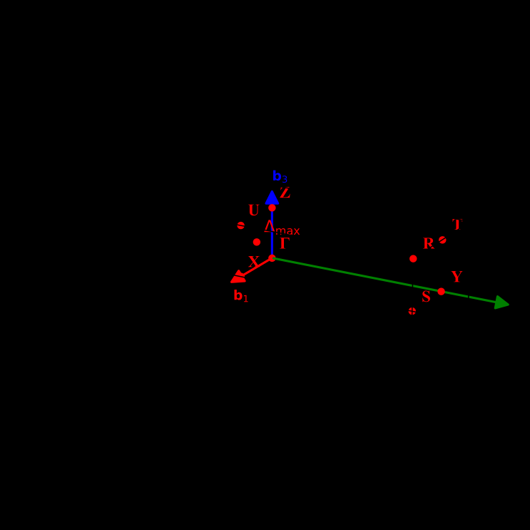
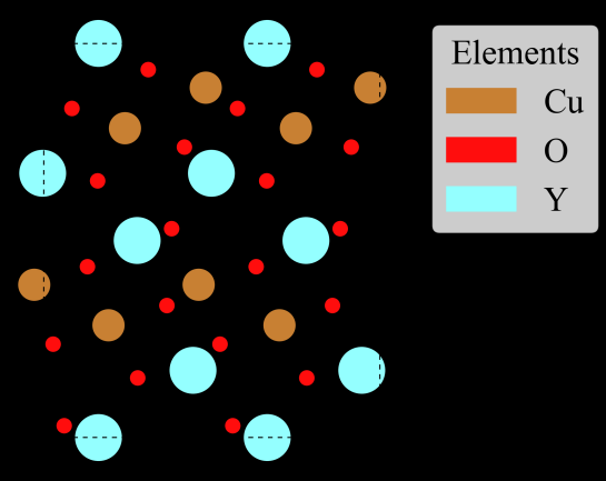
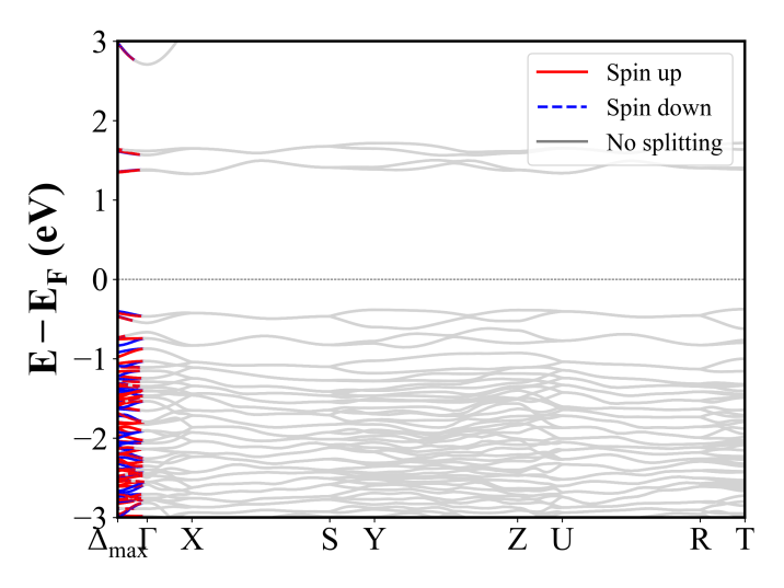
ZnFeH4O2F5 (Imm2) | Band Gap = 3.124 eV
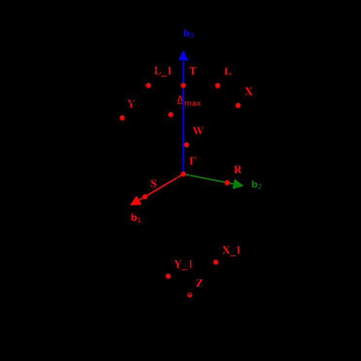
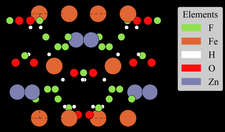
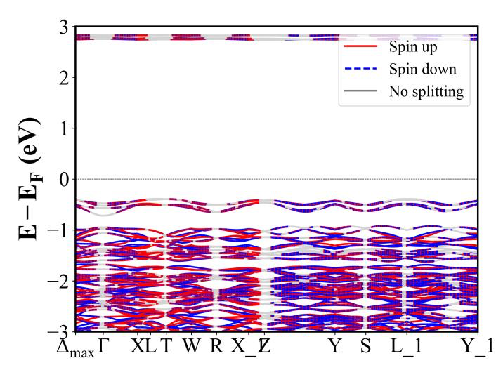
YCrO3 (Pnma) | Band Gap = 3.124 eV
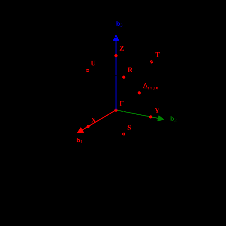
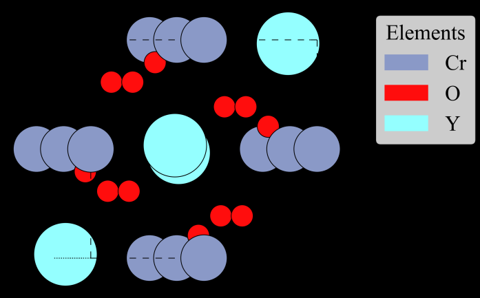
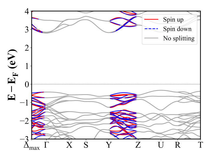
CuH9C4(NO2)3 (Pna2_1) | Band Gap = 2.201 eV
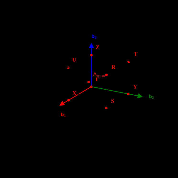
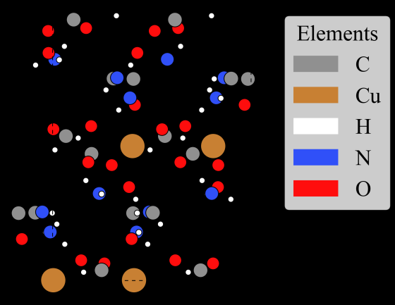
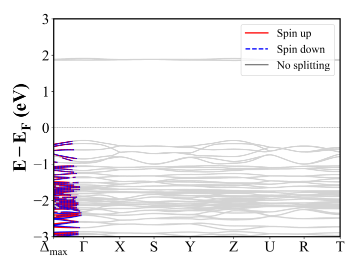
YVO3 (Pnma) | Band Gap = 2.037 eV
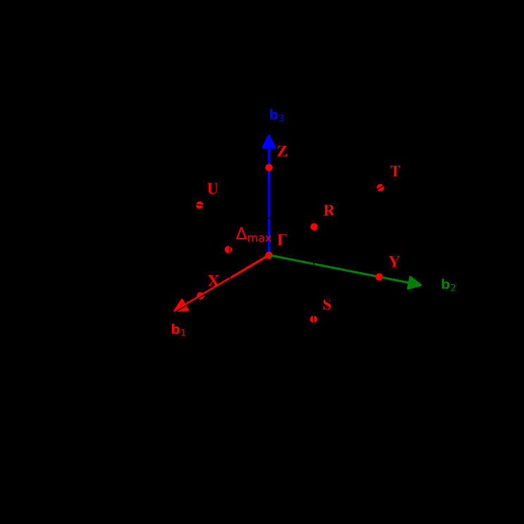
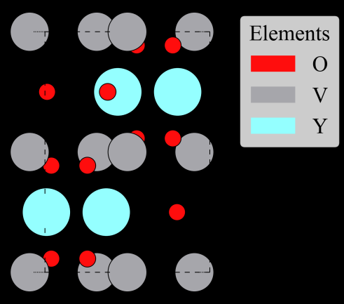
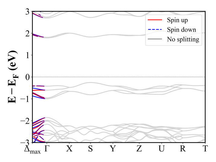
YRuO3 (Pnma) | Band Gap = 0.569 eV
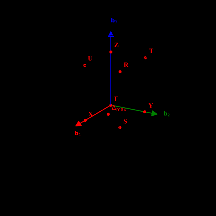
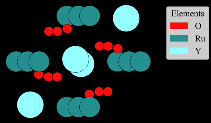
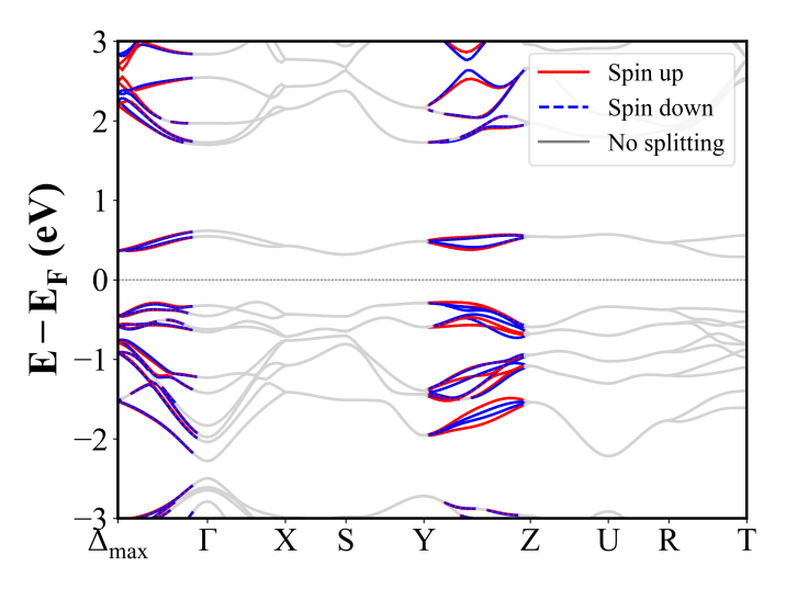
UGaNi (P-62m)
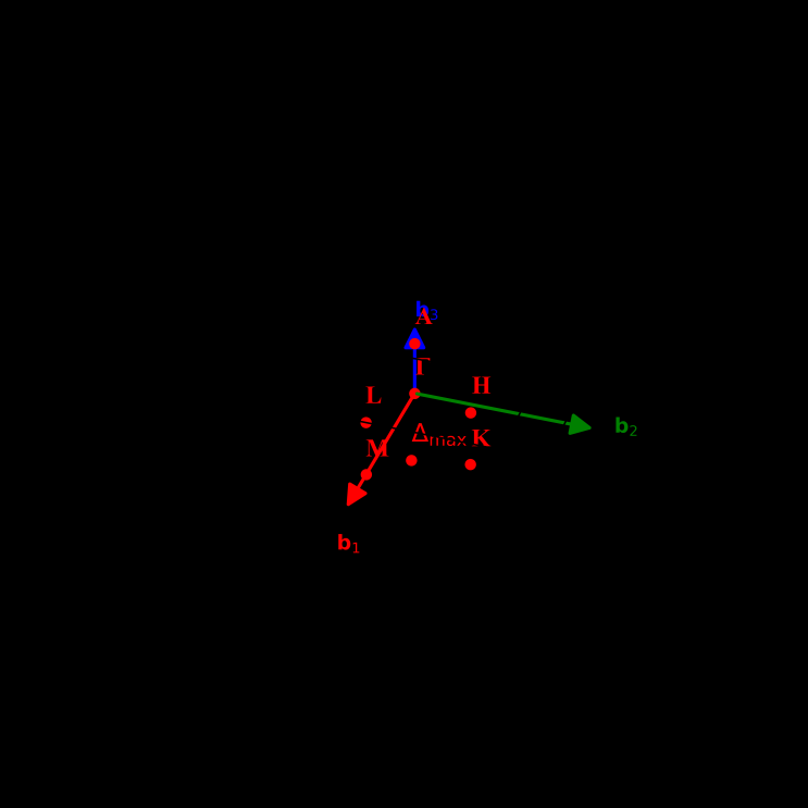
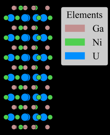
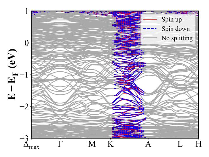
ZrMn2(GeO3)4 (P4/nbm) | Band Gap = 2.309 eV
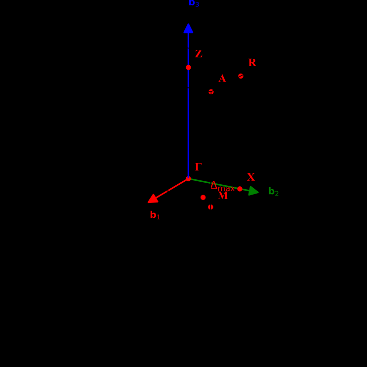
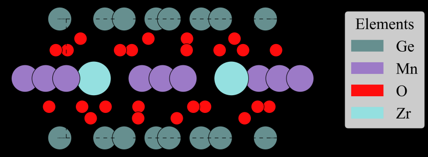
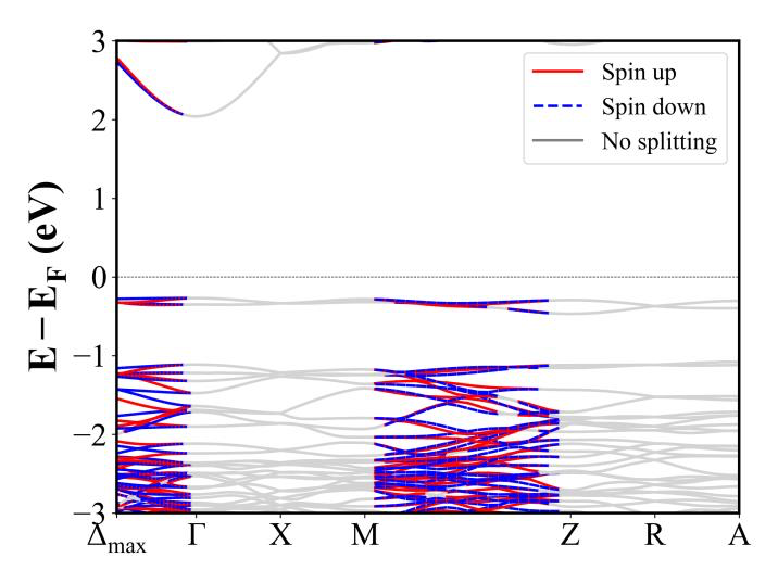
ZrCo2(GeO3)4 (P4/nbm) | Band Gap = 2.628 eV
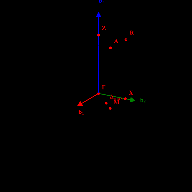
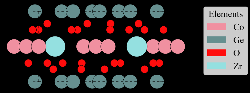
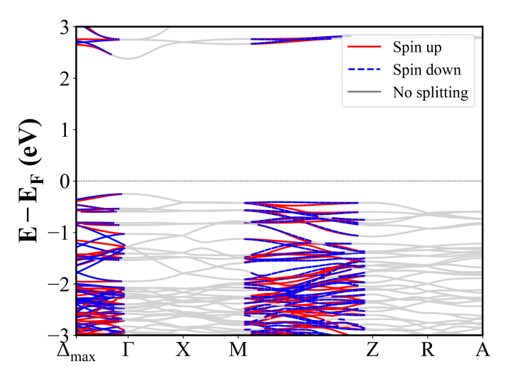
UCr2Si2C (P4/mmm) | Band Gap = 0.000 eV
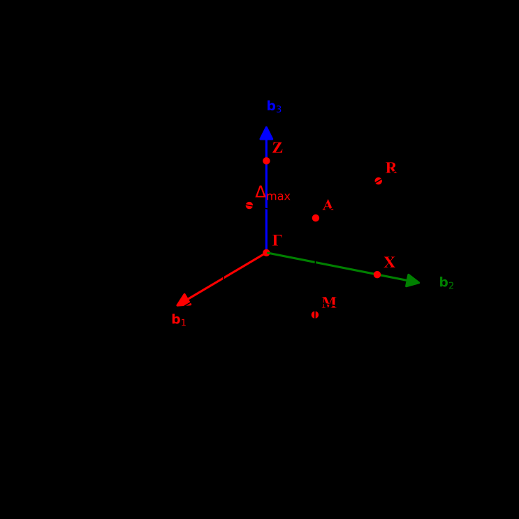
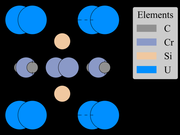
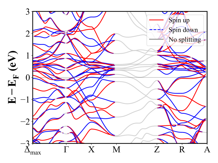
BaCu(TeO3)2 (P4_132) | Band Gap = 1.933 eV
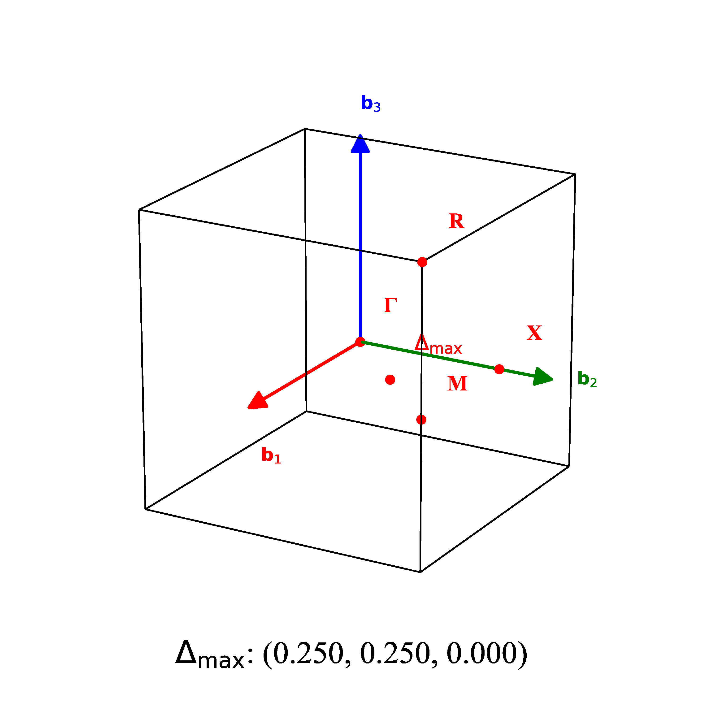
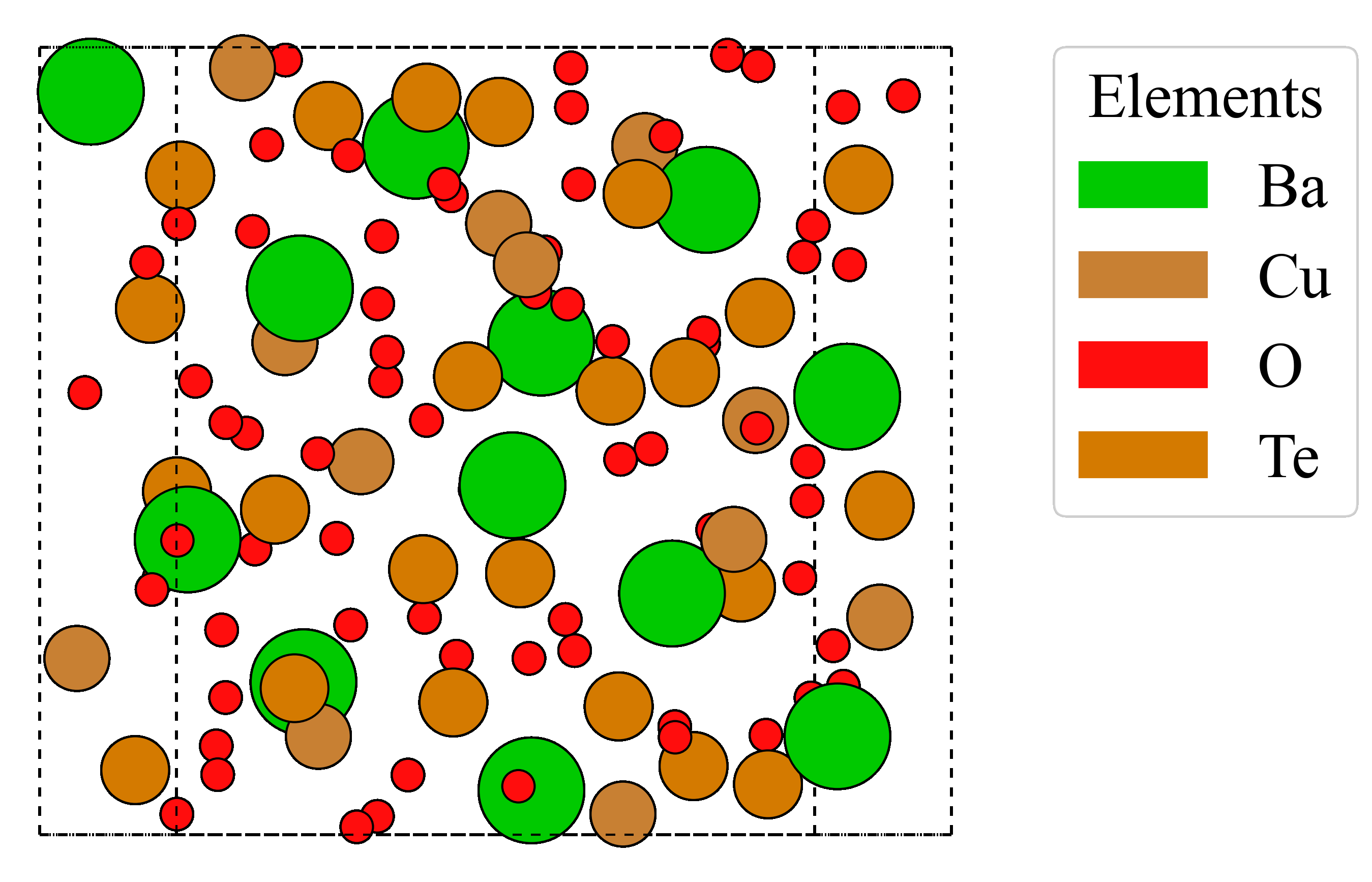
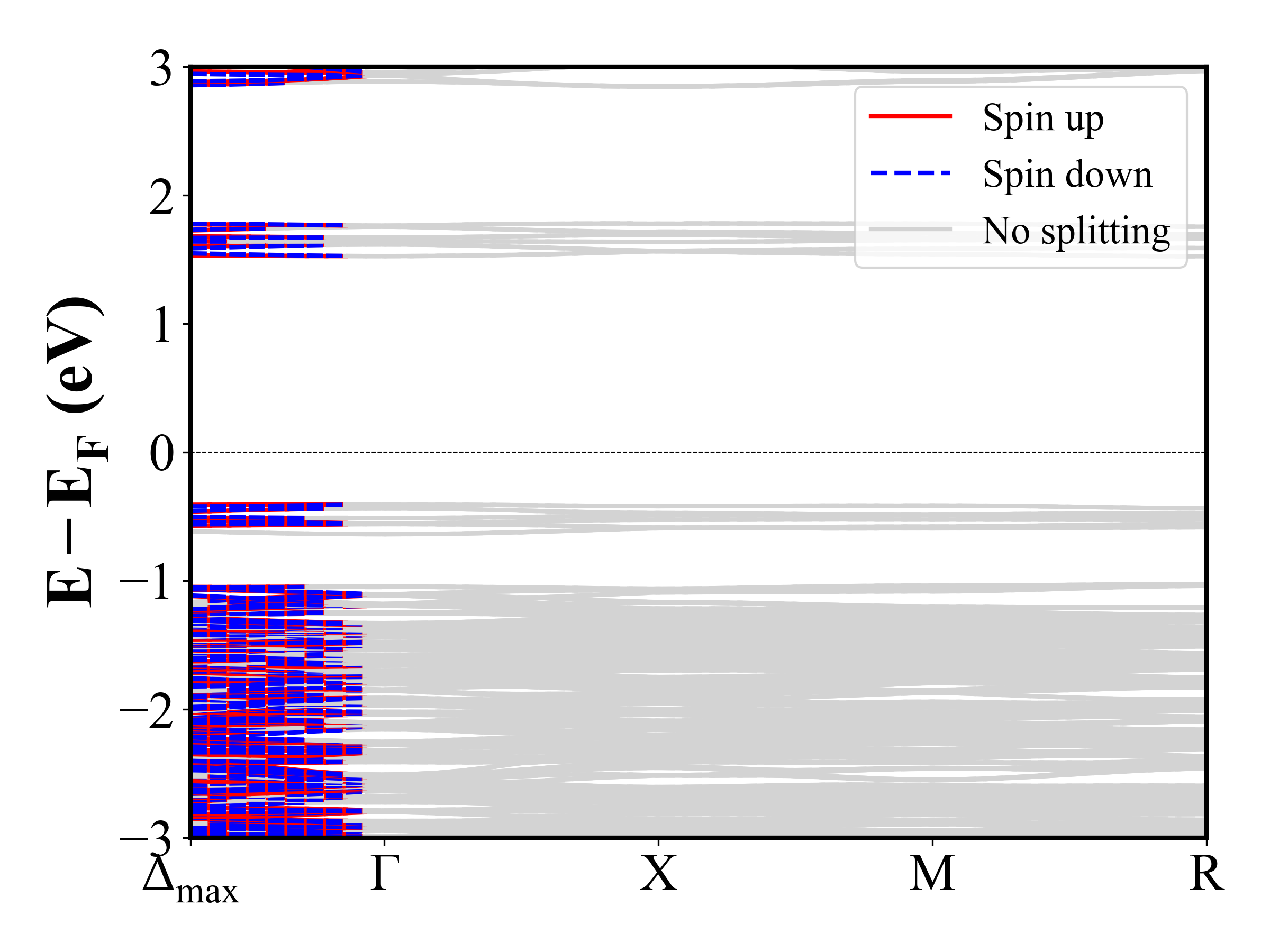
SrCu(TeO3)2 (P4_132) | Band Gap = 1.985 eV
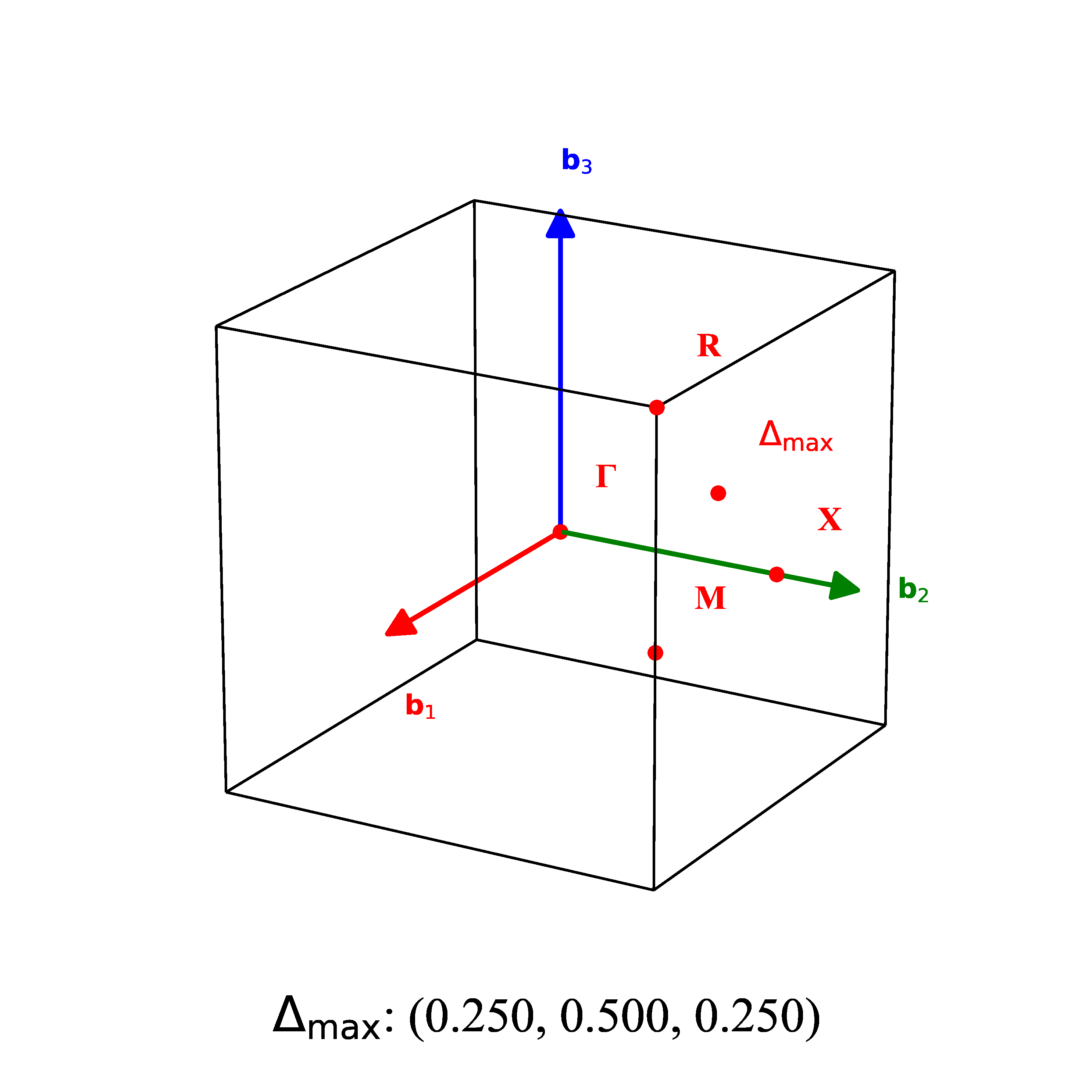
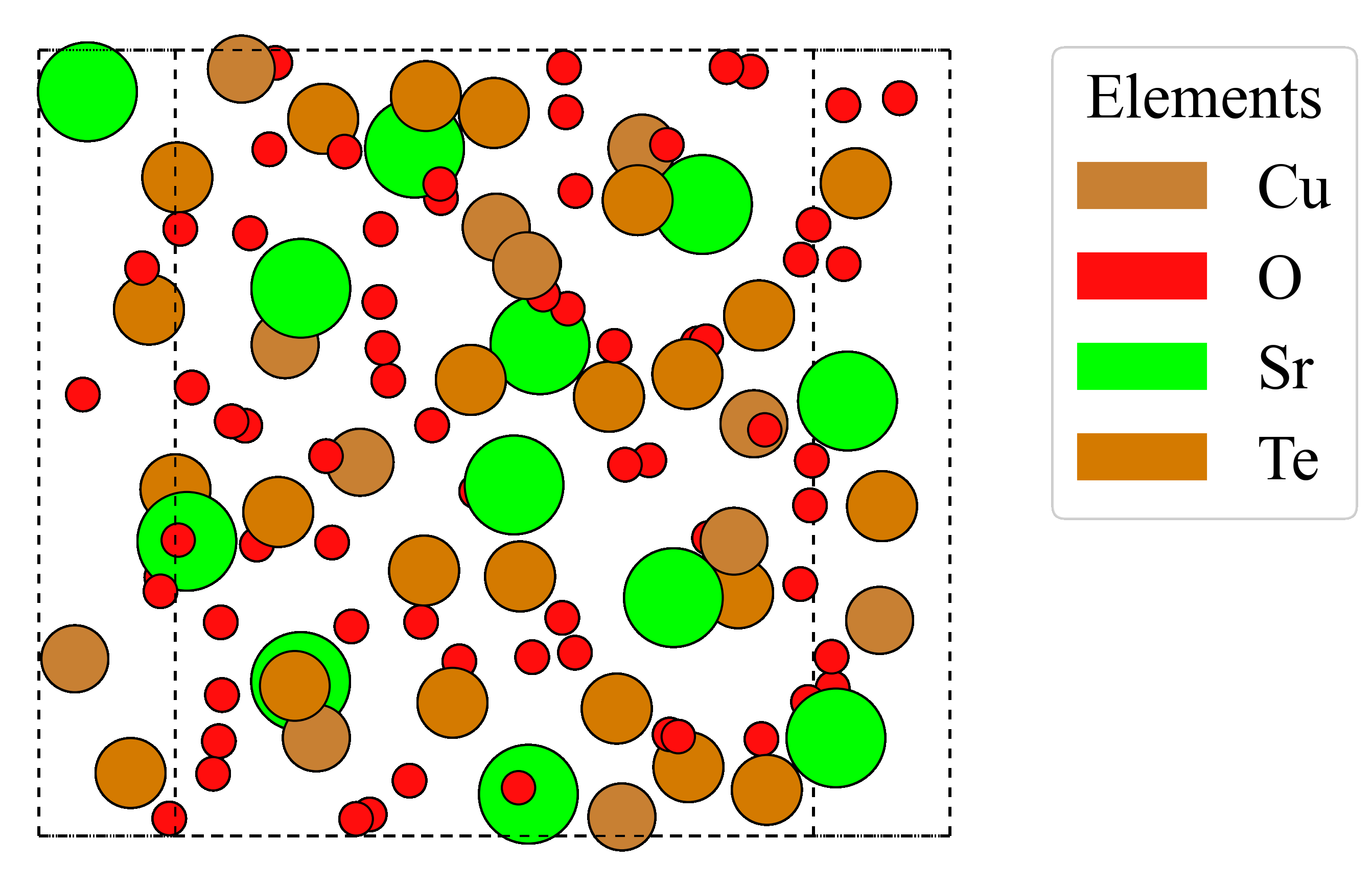
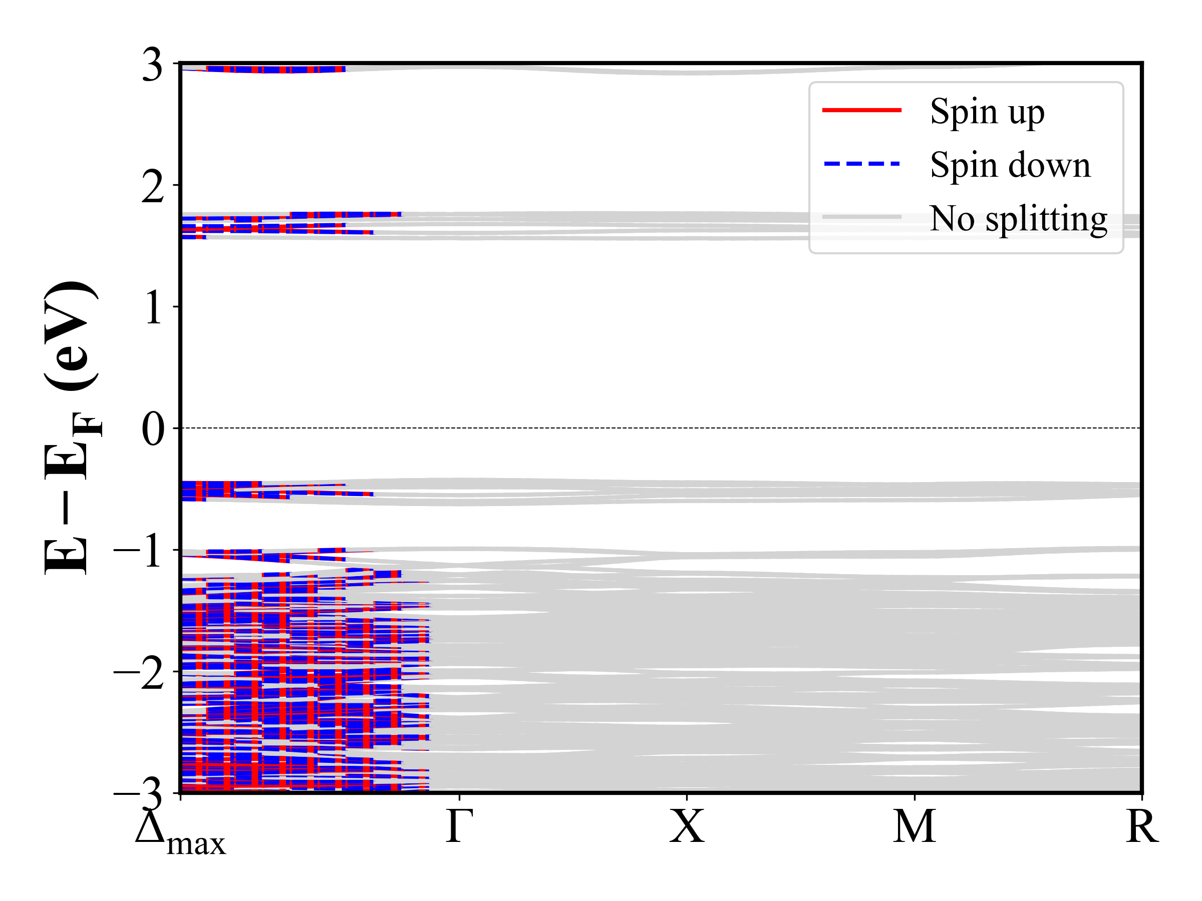
KMnF3 (Pnma) | Band Gap = 4.057 eV
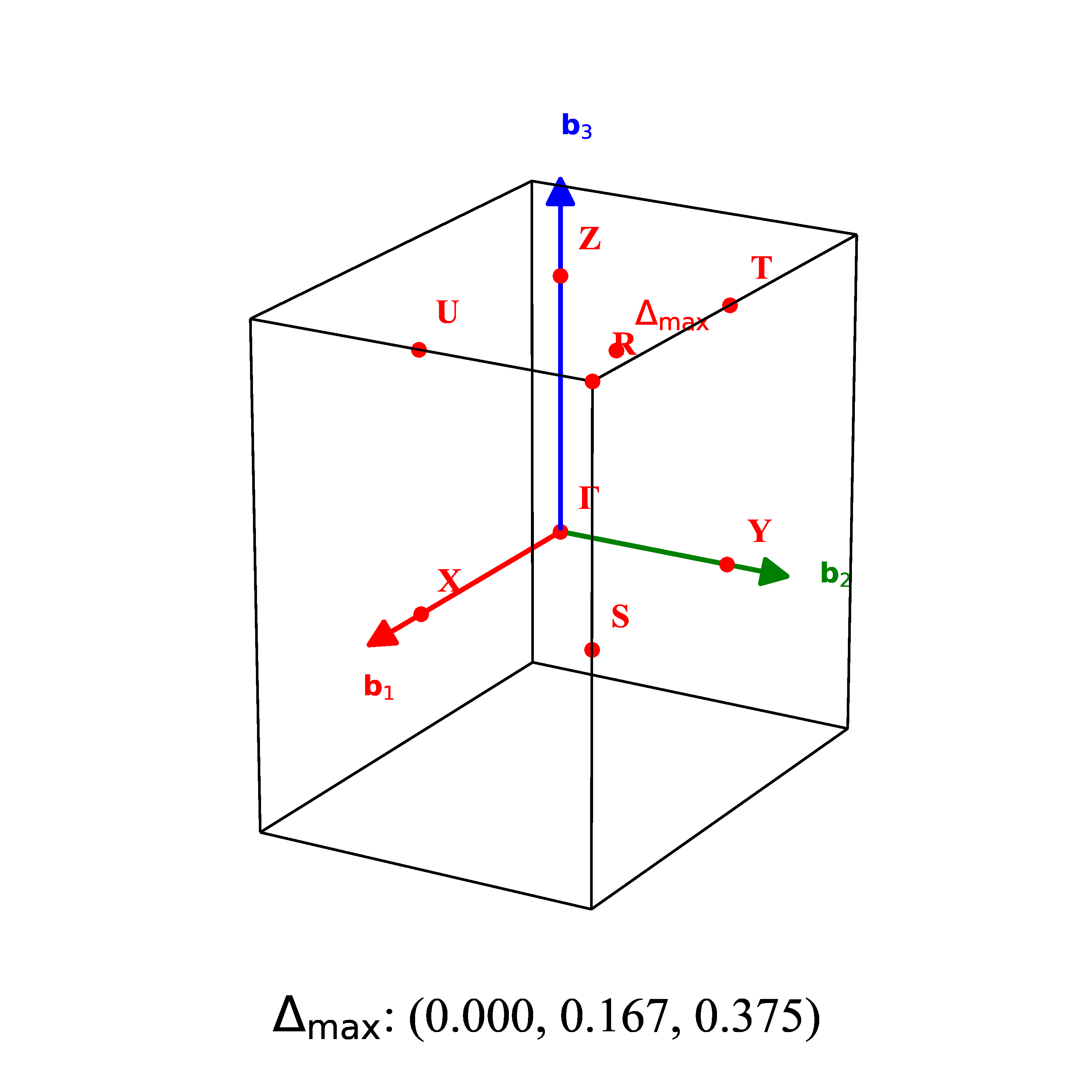
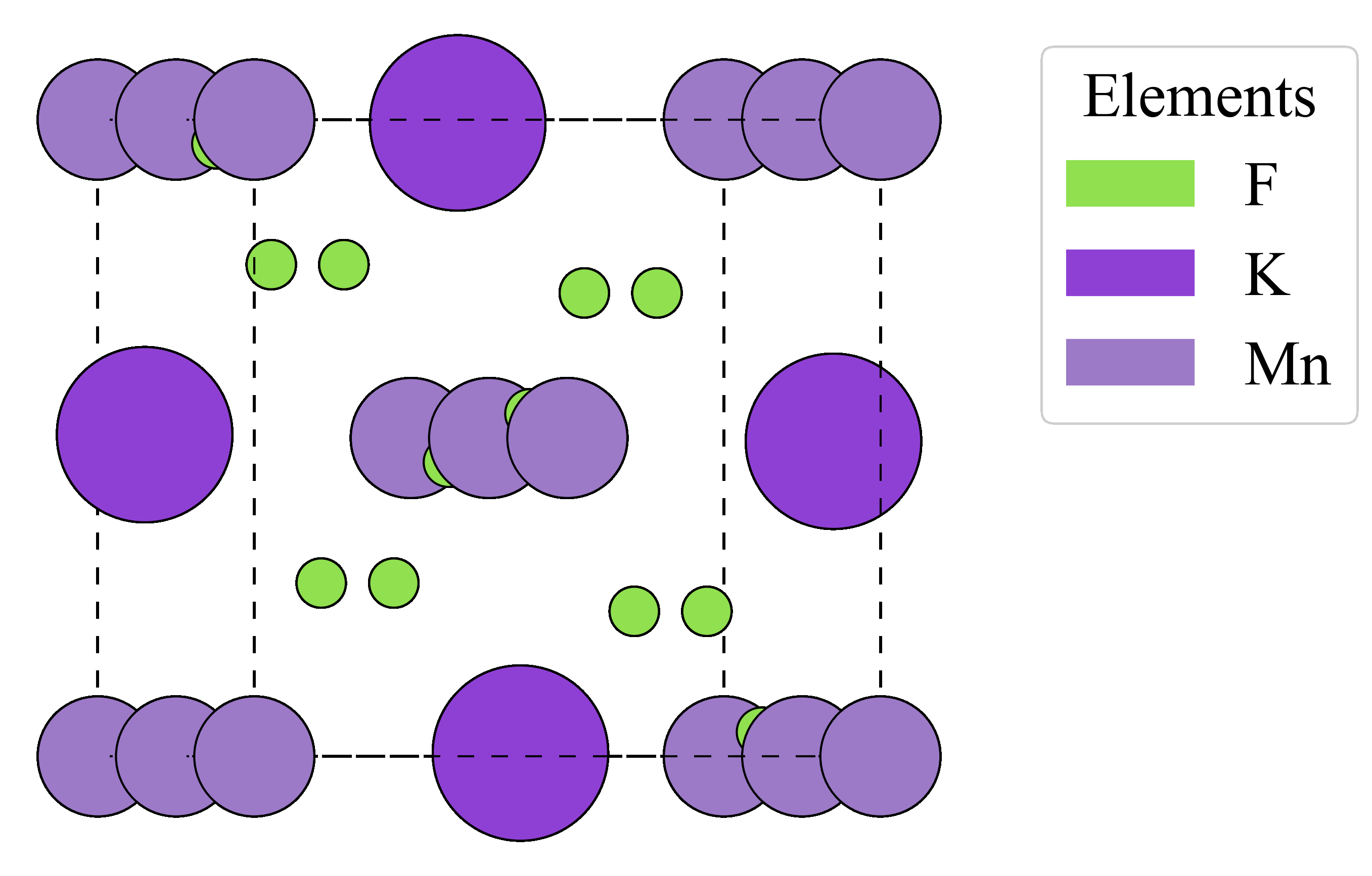
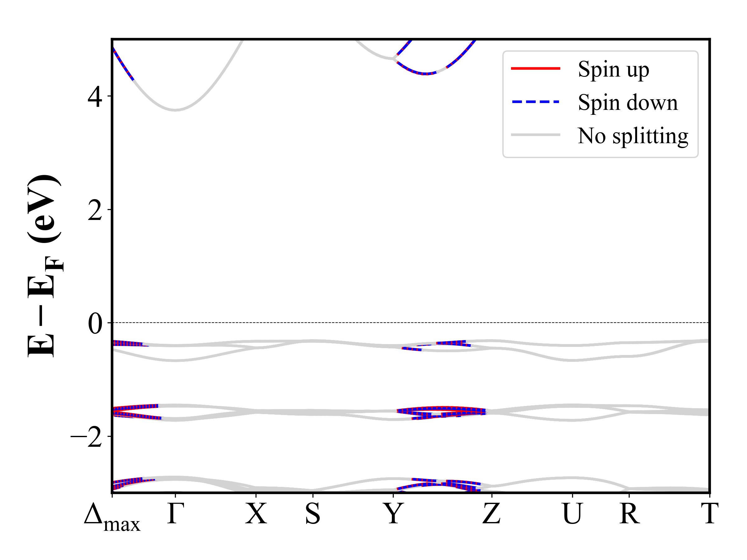
Er5(In2Pd)2 (Pbam) | Band Gap = 0.000 eV
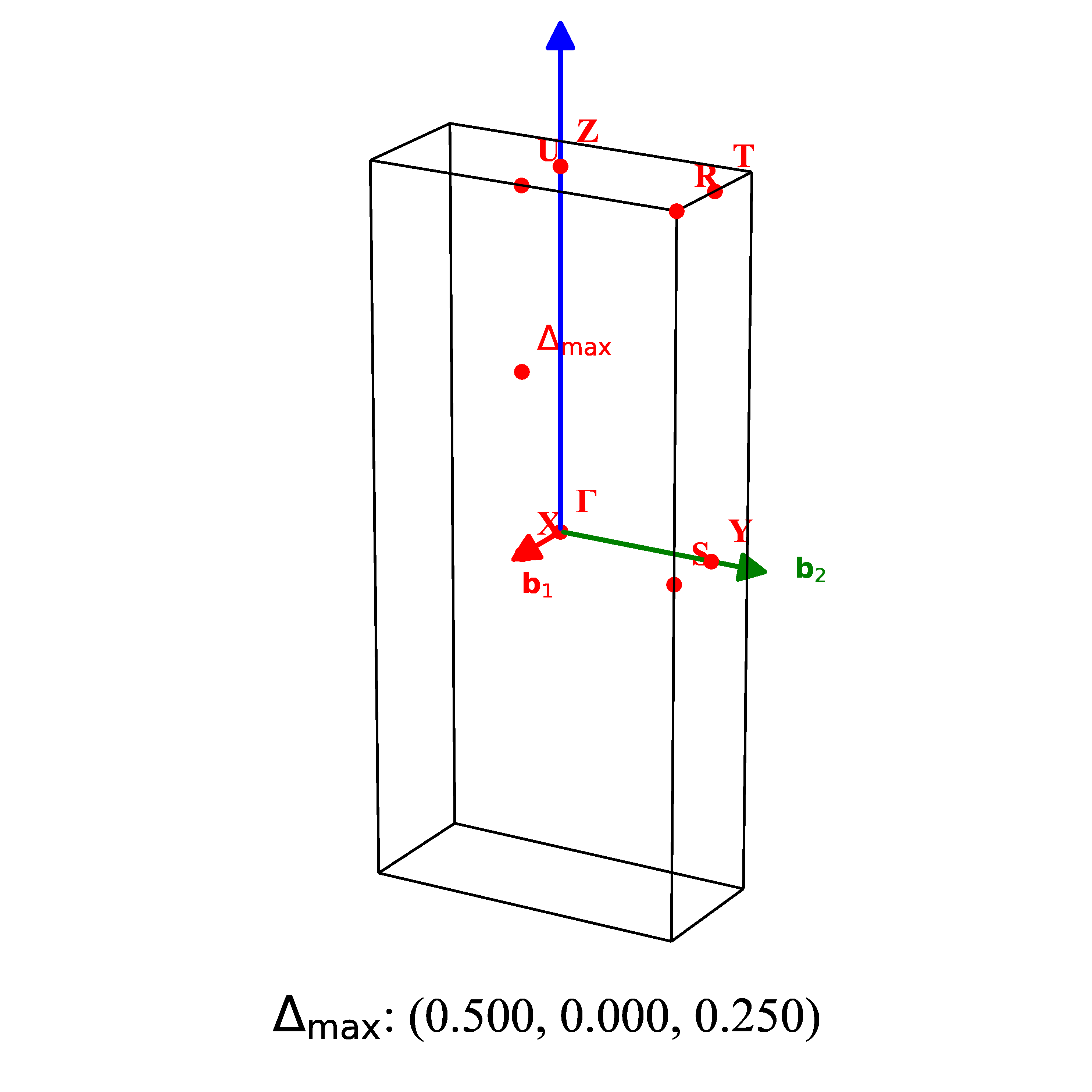
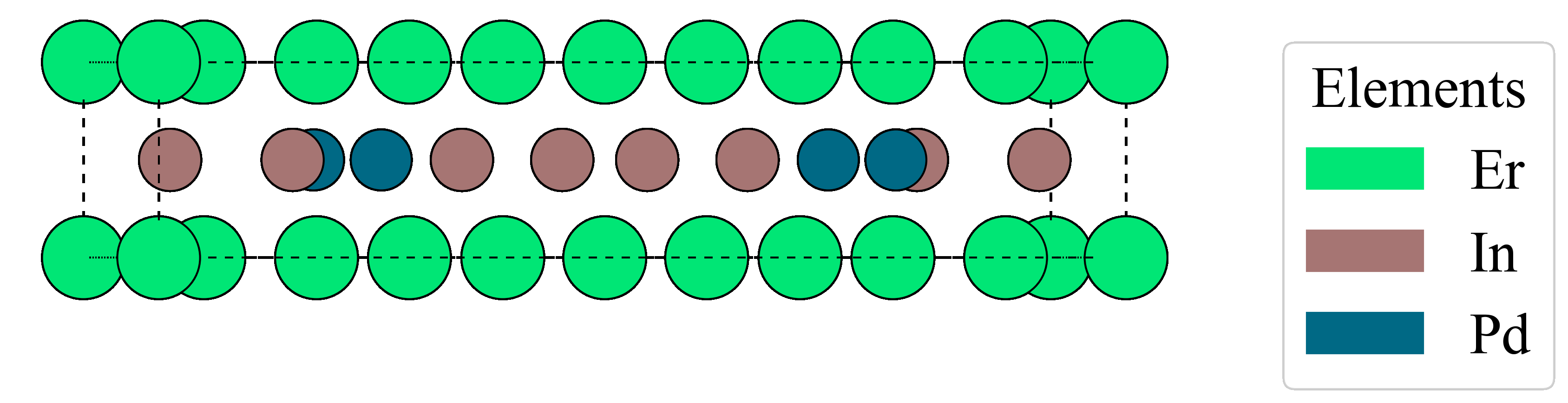
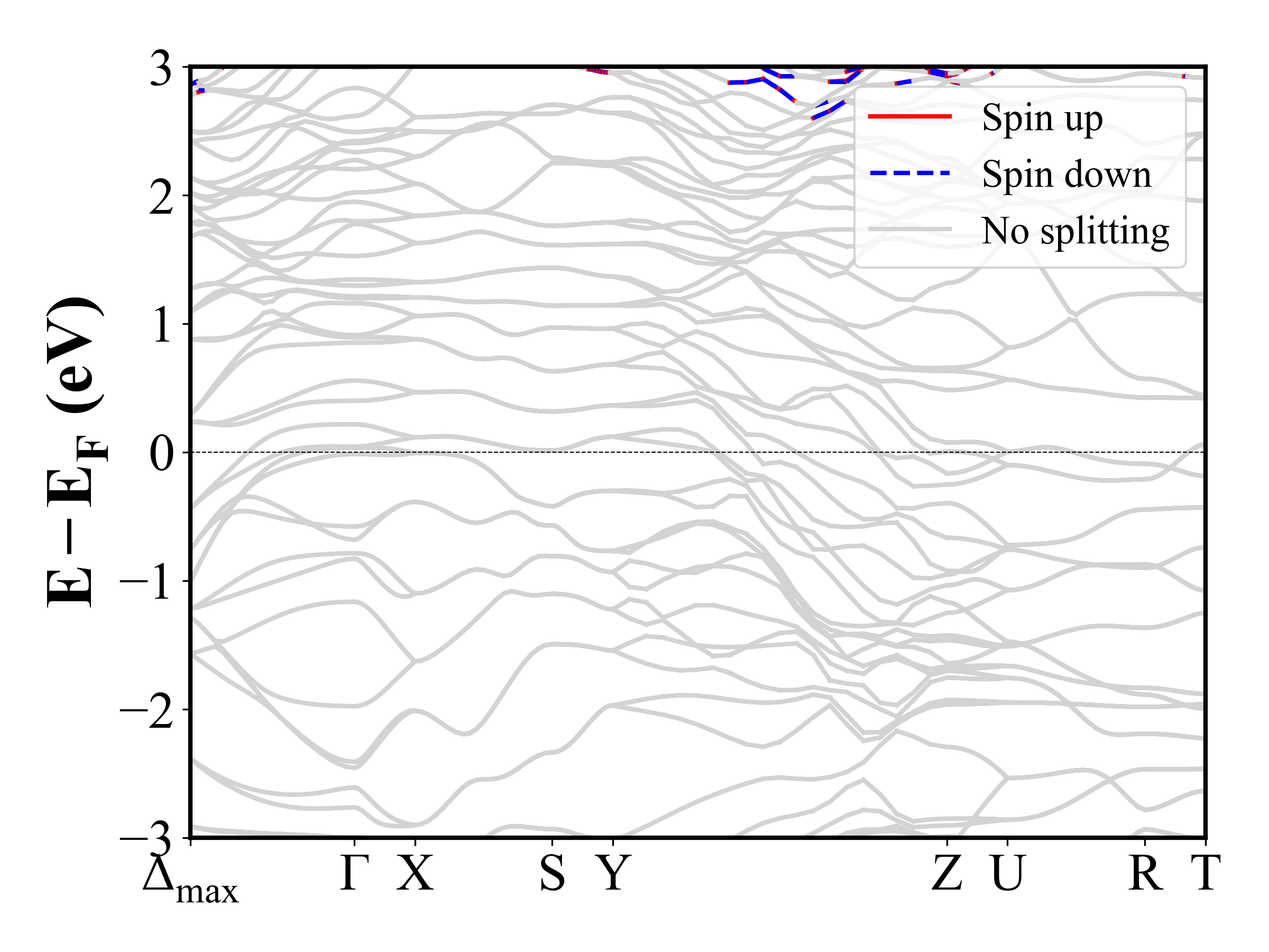
BaCrF5 (P2_12_12_1) | Band Gap = 4.241 eV
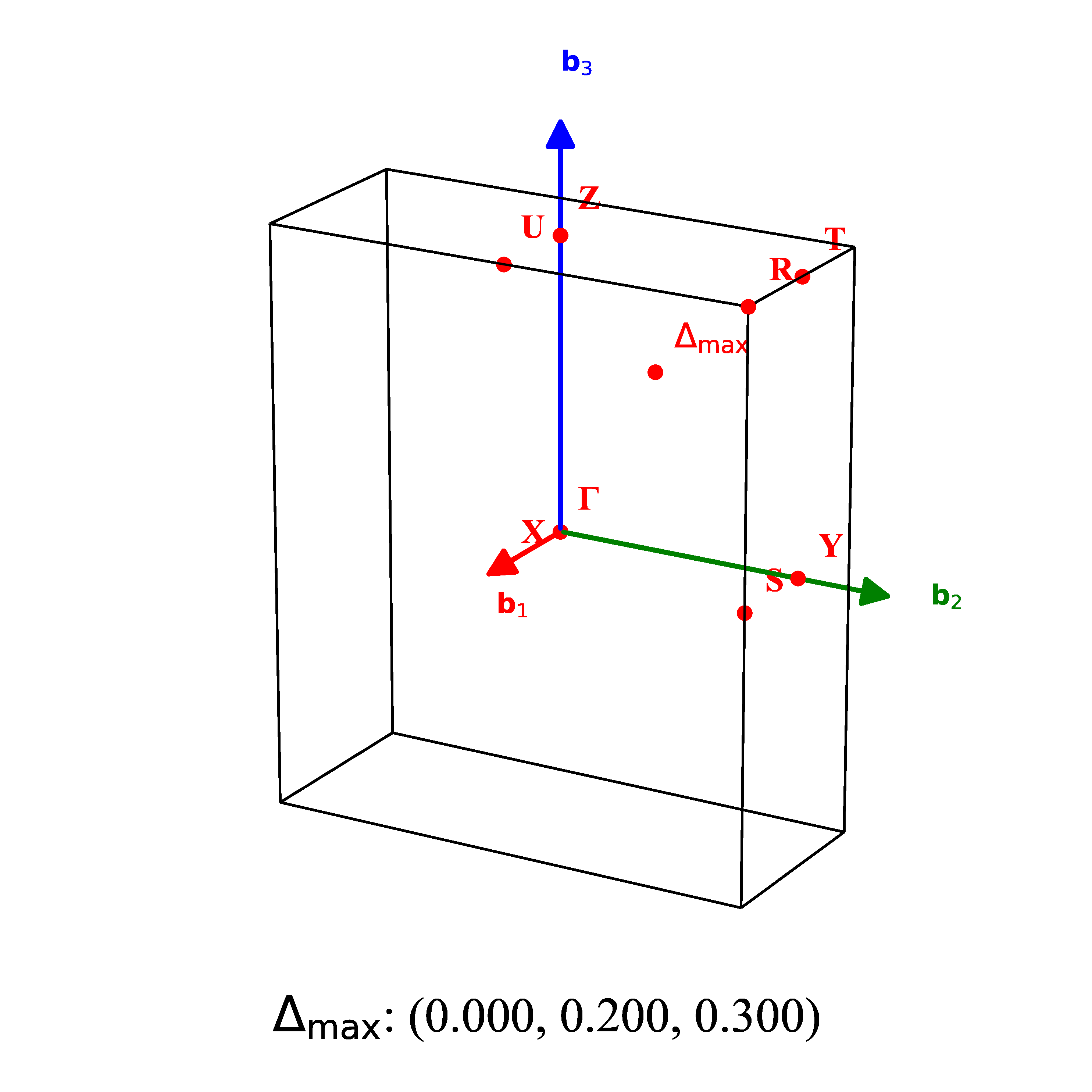
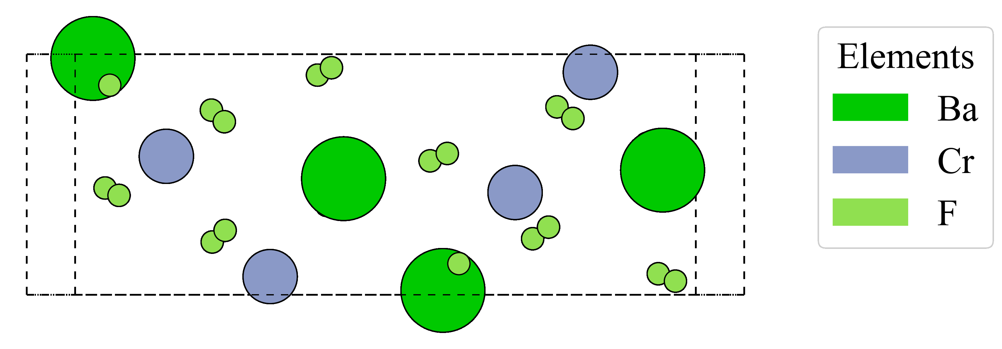
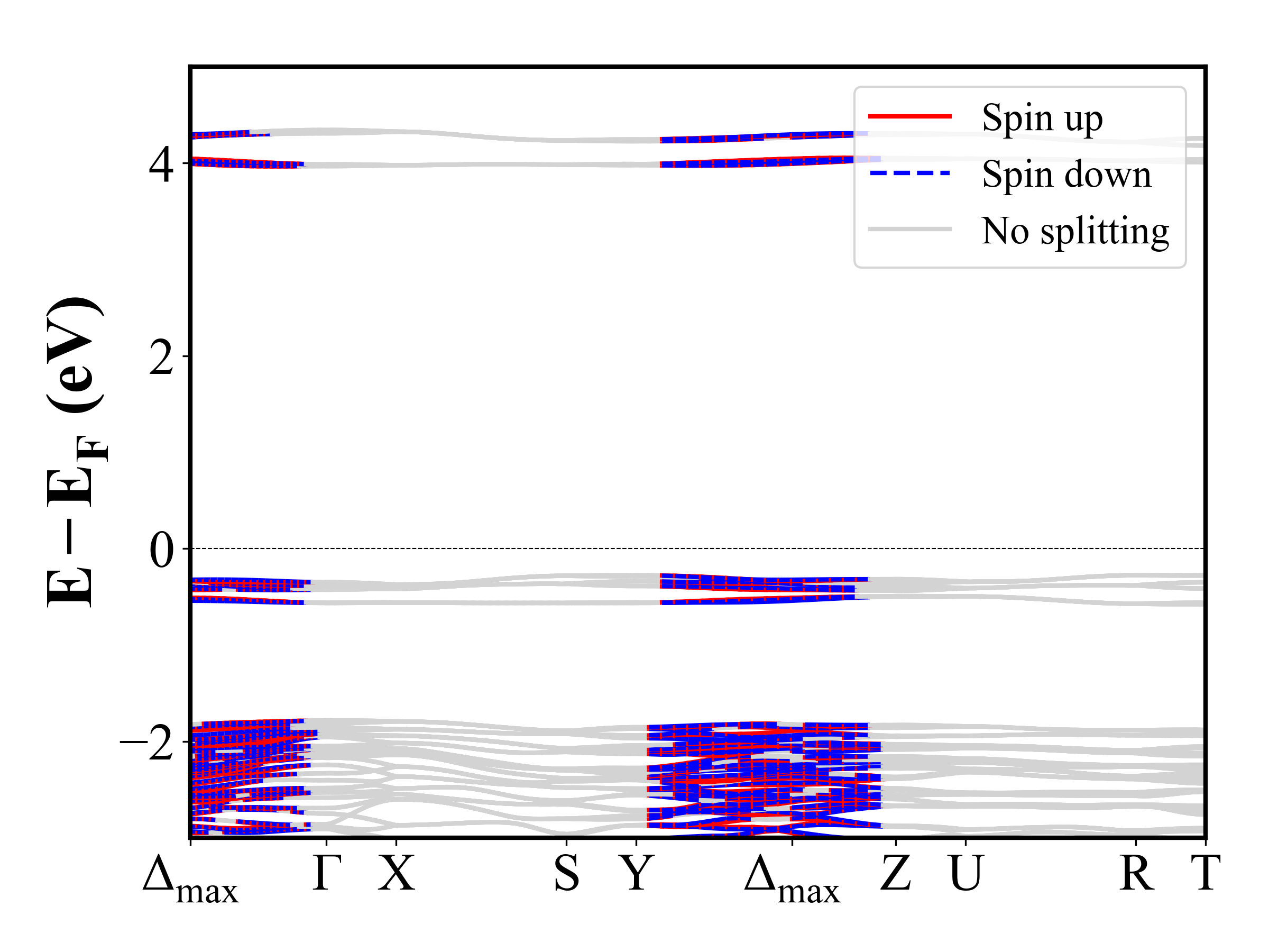
Ba3CoSb2O9 (P6_3/mmc) | Band Gap = 2.479 eV
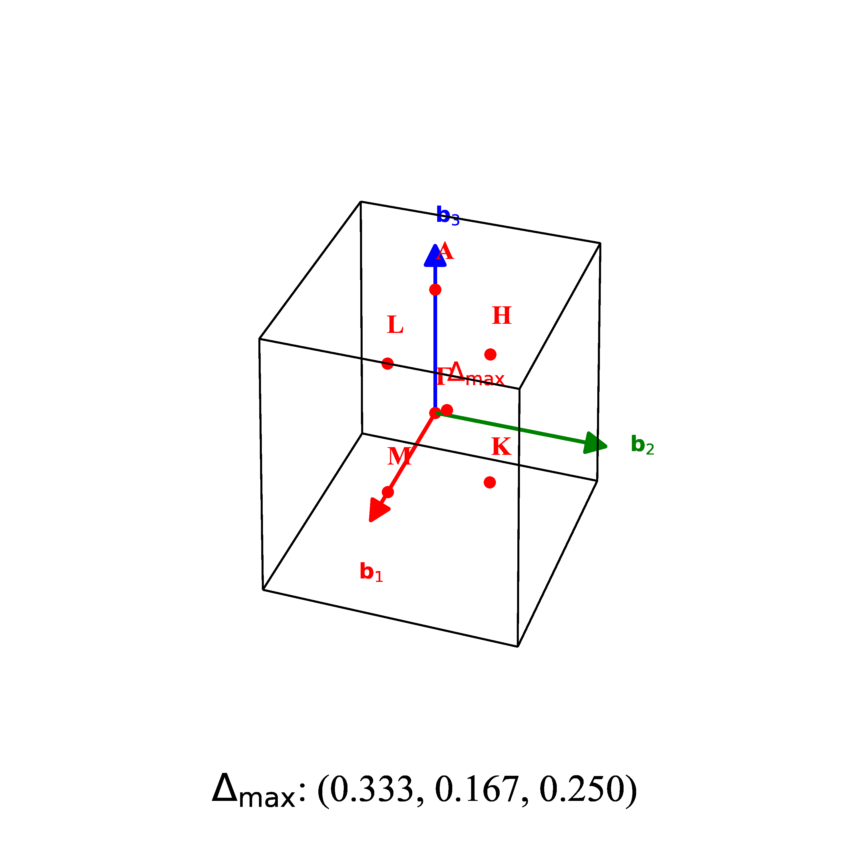
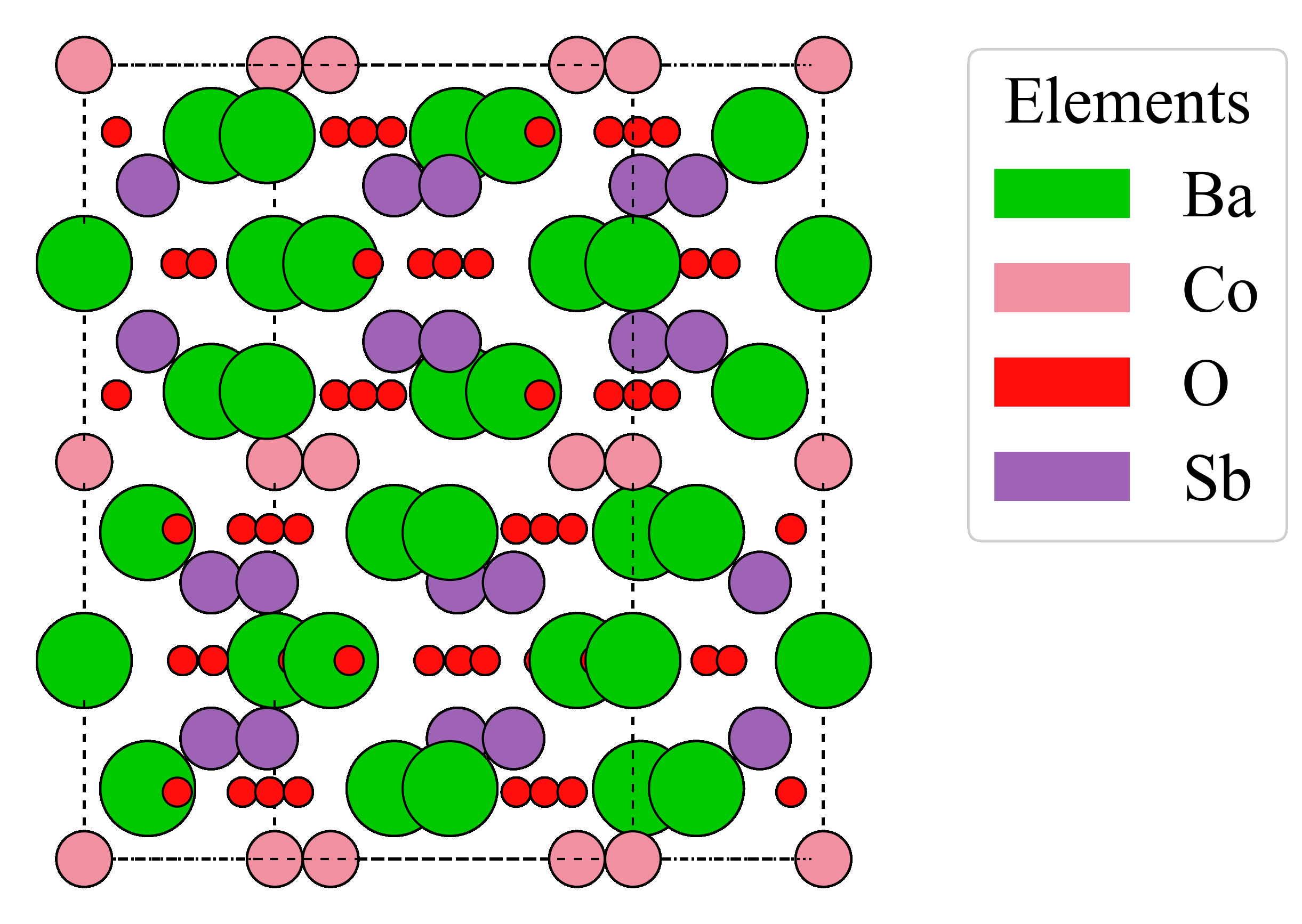
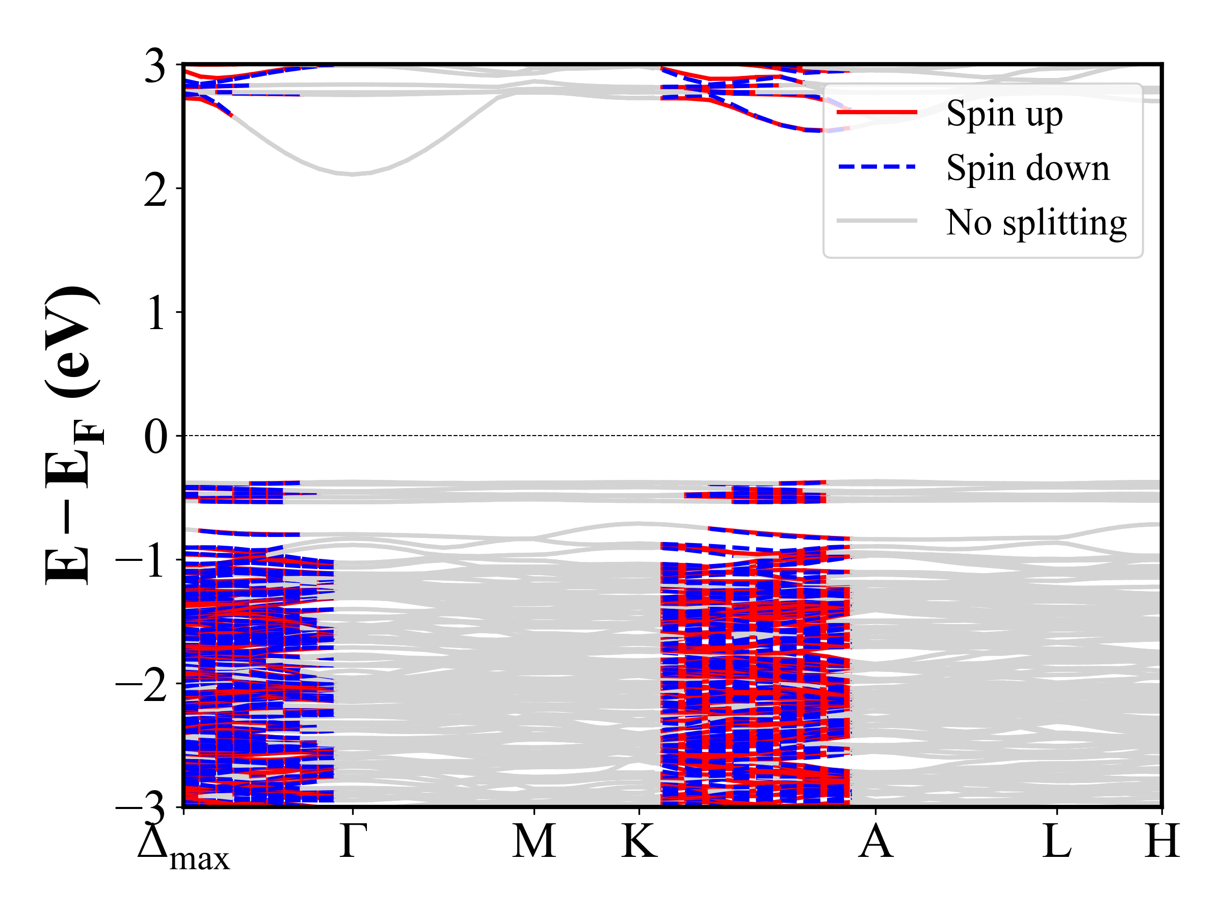
CrH4NF3 (P4_2/mbc) | Band Gap = 2.831 eV
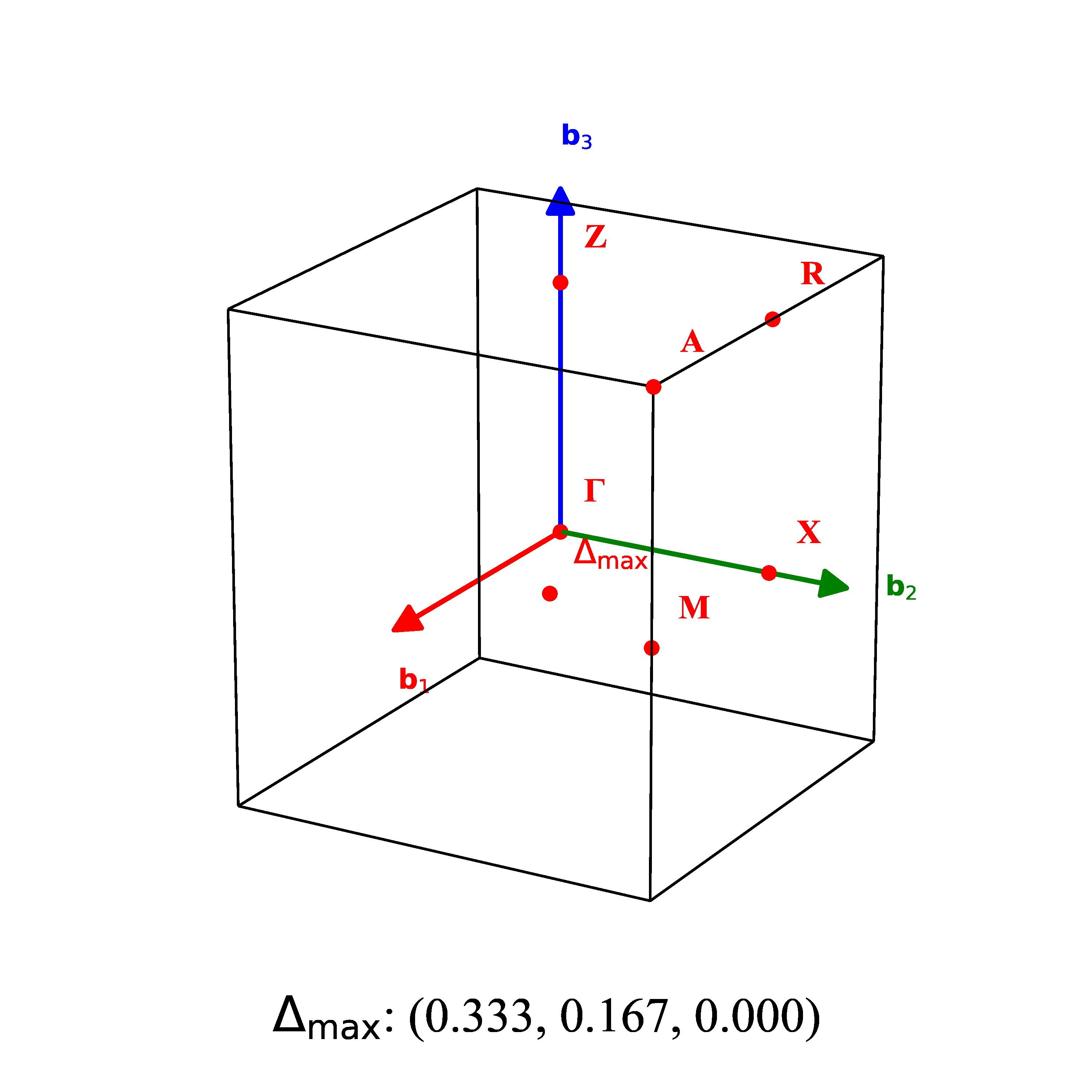
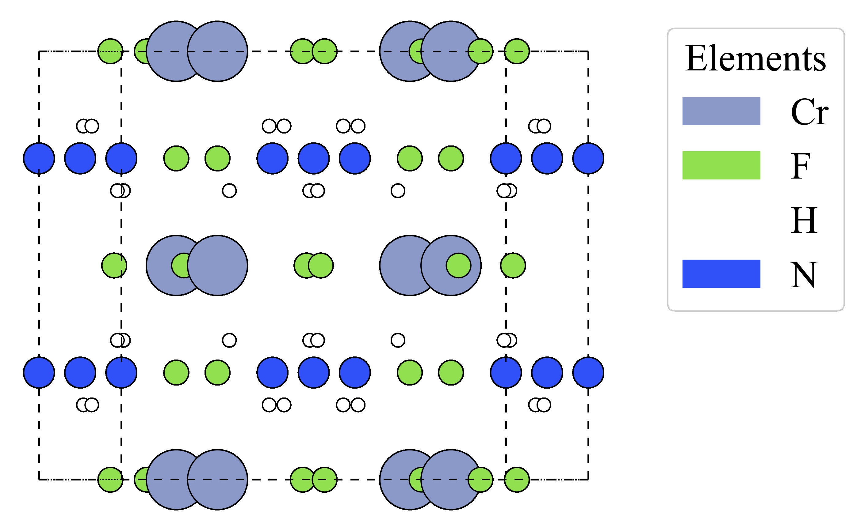
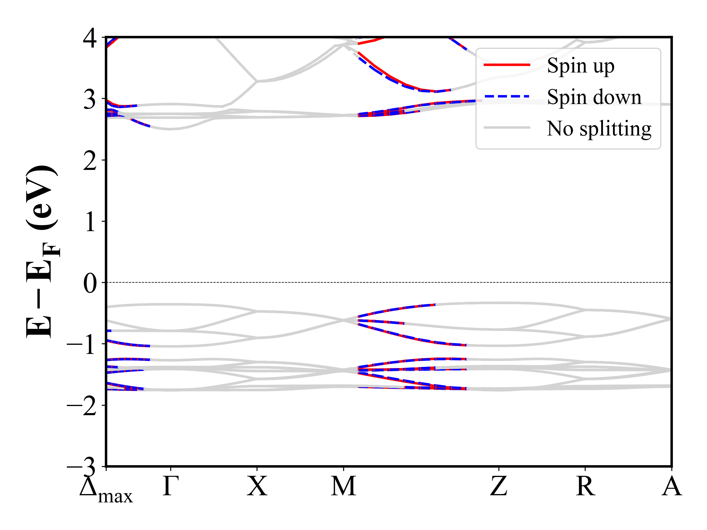
CsNiCl3 (P6_3/mmc) | Band Gap = 3.837 eV
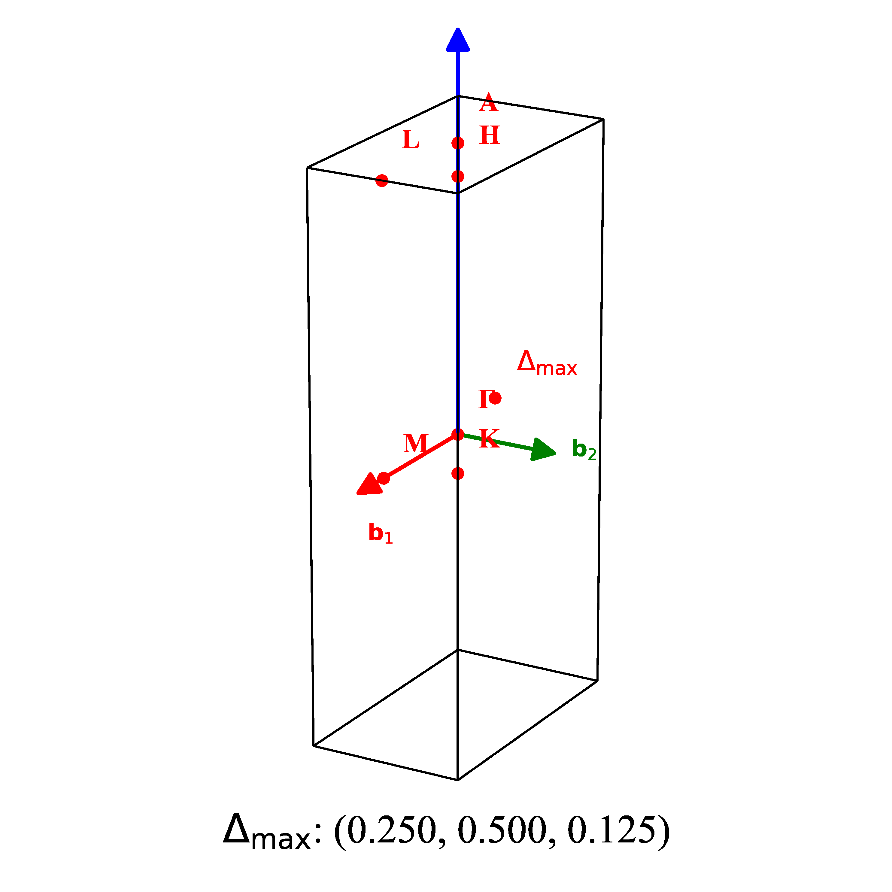
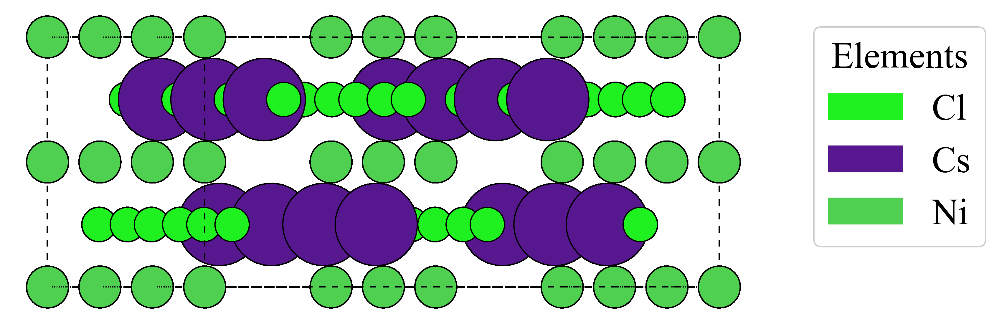
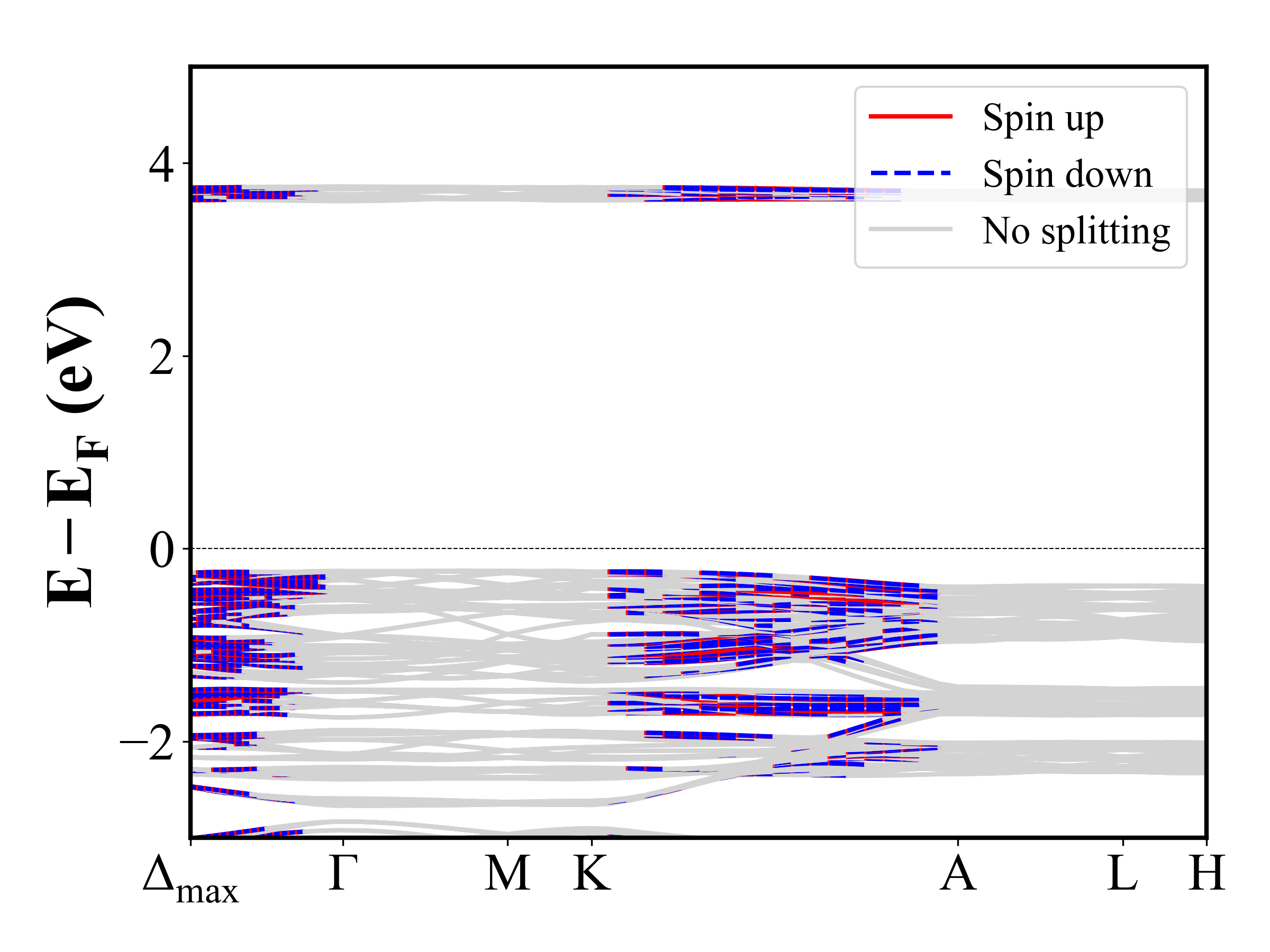
Na2CoP2O7 (Pna2_1) | Band Gap = 3.332 eV
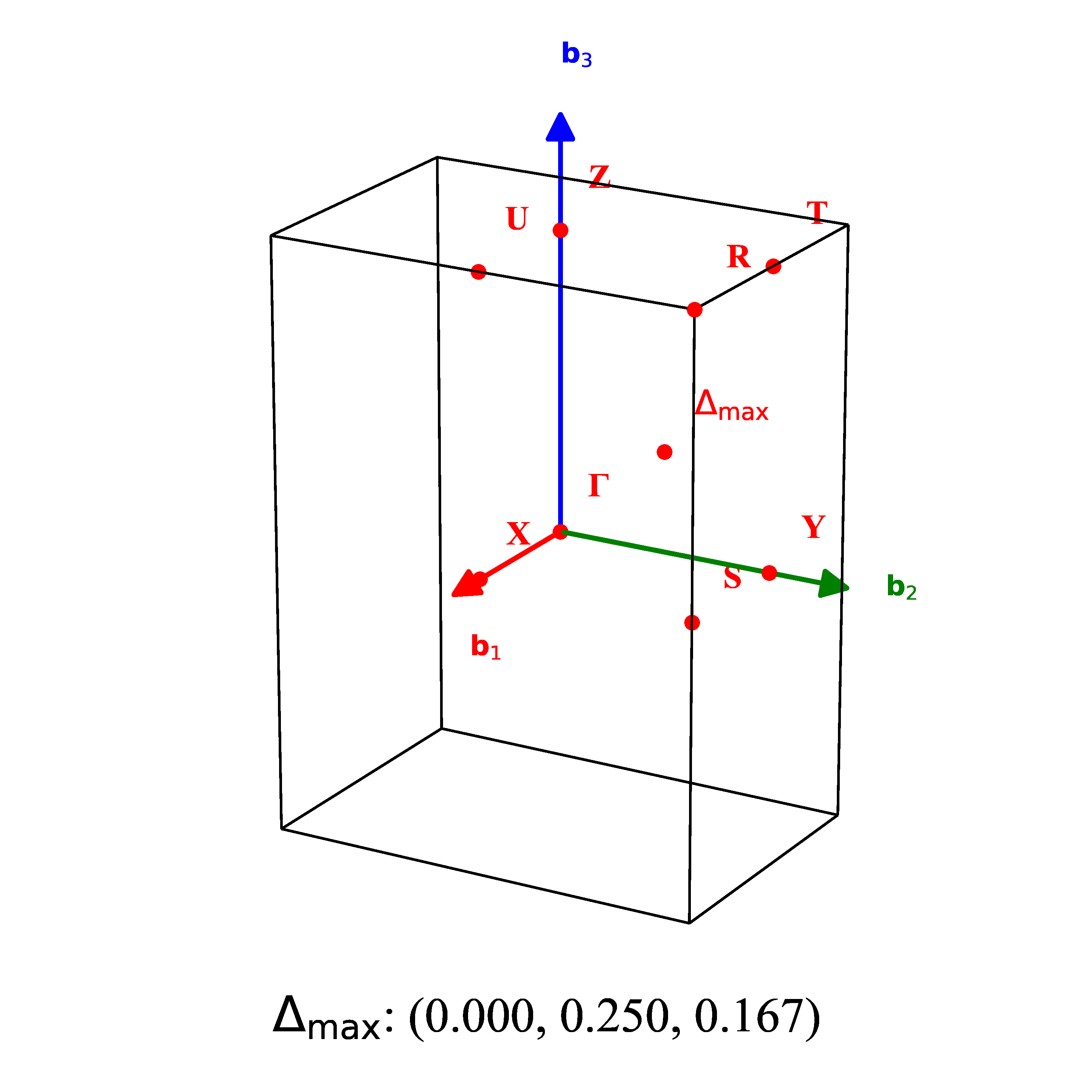
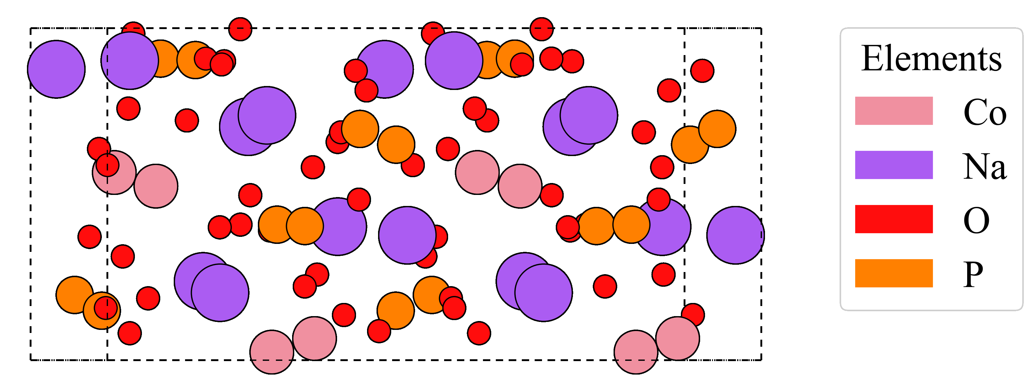
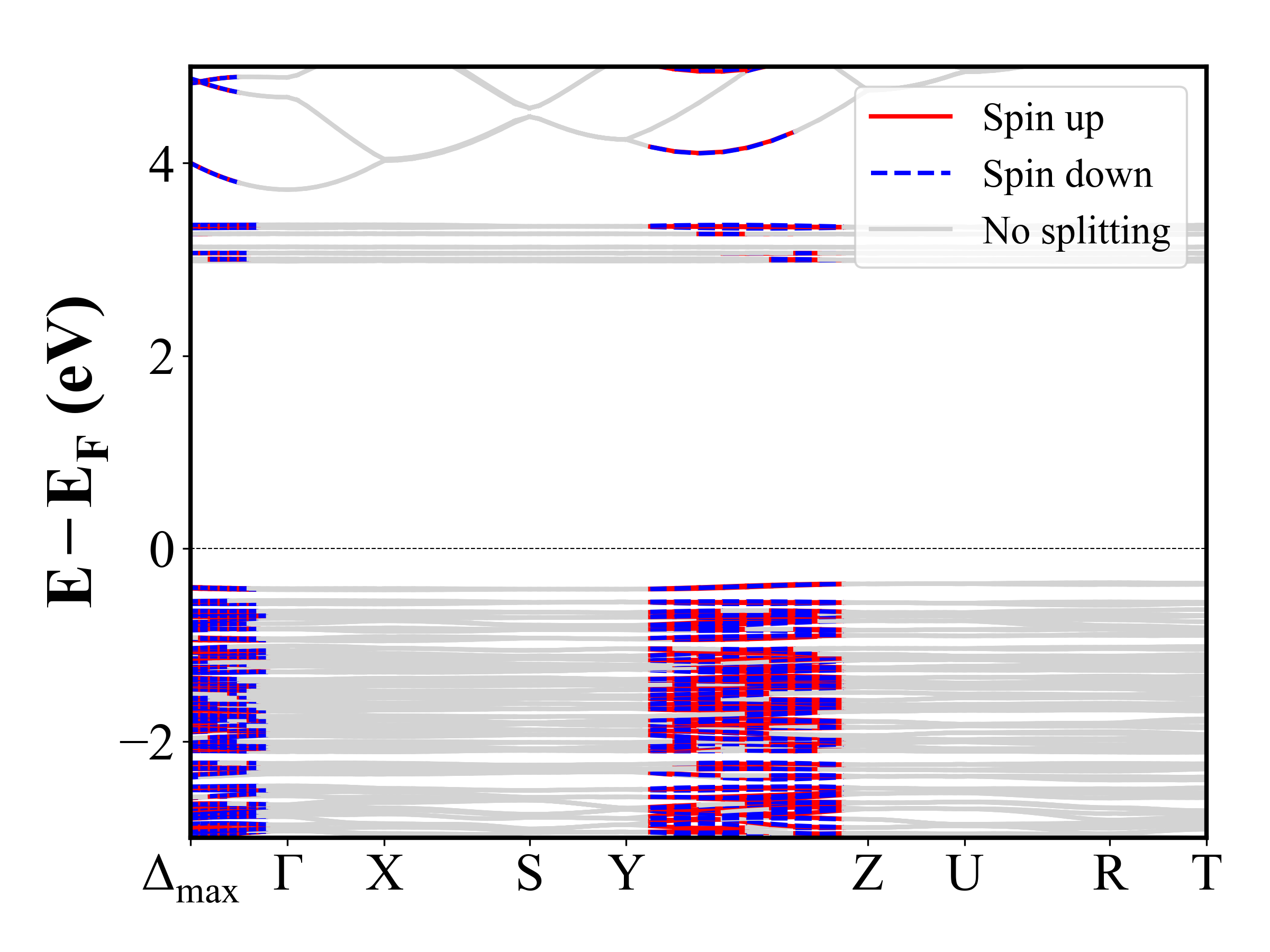
Eu(InAs)2 (P6_3/mmc) | Band Gap = 0.000 eV