⬇ Download Markdown · ⬇ Download LaTeX · ⬇ original · view original · CSV: table 1, table 2
Toru Takahashi a,∗ , Tatsuya Tokito a , Yi Cui a , Toshiro Matsumoto a
a Department of Mechanical Systems Engineering, Nagoya University, Furo-cho, Chikusa-ku, Nagoya city, Aichi, 464-8603 Japan
Abstract
This paper introduces a shape optimisation framework for achieving desired mutual inductances (MIs) among coils in 3D space. Utilising a wire modelling approach, the coils are discretised using B-spline curves, with control points (CPs) serving as design variables. The key contribution is the derivation of the shape derivative of the objective function in terms of MIs, enabling the use of gradient-based quasi-Newton optimisation methods. A coil length constraint is also incorporated. The study demonstrates the effectiveness of the framework through numerical examples, validating the theoretical and numerical developments. This approach addresses the largely unexplored area of magnetostatic MI optimisation within the wire modelling framework, offering a computationally efficient alternative to finite element methods etc. Keywords: Mutual inductance, B-spline function, Shape optimisation, Shape derivative, Biot–Savart law, Nonlinear programming
Mutual inductance (MI) plays a pivotal role in a wide range of devices, including transformers, wireless power transfer systems, and near-field sensors. Enhancing the performance of these devices necessitates accurate analysis and optimisation of MIs among coils. Coils are typically modelled either as infinitely-thin wires carrying a prescribed current (scalar), or as finite-volume conductors with a current density (vector field) determined by Maxwell’s equations. While the latter approach more accurately captures coil geometry, it entails significant computational complexity and cost due to the use of numerical methods like the finite element method (FEM).
In contrast, the simplified wire model offers a computationally efficient alternative. The Biot–Savart (BS) law, expressed as a contour integral, enables direct calculation of the magnetostatic field given the coil shape and current [1]. This approach has been extensively used to investigate MIs in various coil configurations. For instance, Kim et al. [2] computed the MI of spiral coils, Boissoles et al. derived the MI for bird-cage coils using integral forms and Gaussian quadrature, and Sonntag et al. [3] examined a formula to calculate MI between planar printed circuit boards (PCBs). Akyel et al. [4] studied the MI of circular and square coils based on Grover’s formula [1] and a numerical evaluation of the BS law. Joy et al. [5] numerically evaluated the BS law to calculate the MI between two square coils in air when they are placed with various misalingnments; a similar investigation is found in the paper by Zhang et al. [6]. Further research by Cheng et al. [7], Paese et al. [8], and Itoh et al. [9] explored MIs in various coil geometries, including spiral rectangular and toroidal-field coils.
Meanwhile, it should be noted that wire models are not always applicable, especially when dealing with skin effects and low-frequency time-varying electromagnetic fields. Numerical models (e.g., using finite elements with appropriate discretisations to manage the eddy current problem and the high field gradients near the conductor’s surface [10, 11]) are required in these instances to account for such effects.
Optimisation of MIs has been addressed using both bulk and wire modelling. Bulk modelling approaches, often employing commercial FEM solvers, have been applied in neuromodulation [12] and wireless power transfer ∗ Corresponding author Email address: [email protected] (Toru Takahashi)
Preprint submitted to Applied Mathematical Modelling June 18, 2025 [13]. Wire modelling has seen more widespread use [14, 15, 16, 17], typically involving lumped-element models with electromagnetic and geometrical parameters as optimisation variables. Notably, these optimisation studies [12, 13, 14, 15, 16, 17] have primarily focused on frequency-domain dynamics.
However, magnetostatic MI optimisation within the wire modelling framework, the focus of this paper, remains largely unexplored. A related study by Hurwitz et al. [18] utilised a Fourier expansion of coil geometry, treating the coefficients and current as design variables. These coefficients are analogous to the control points (CPs) used here. Nevertheless, their work did not optimise MIs directly.
This study builds upon the first author’s recent work [19] on gradient coil optimisation for MRI, which focused on generating linear magnetostatic fields. Here, the aim of this study is to optimise MIs to target values. To achieve this, coils are approximated with B-spline curves and their CPs are exploited as the design variables. Our primary contribution is the novel derivation of the shape derivative (or shape sensitivity) of MIs with respect to these B-spline control points. This critical development enables the use of powerful gradient-based quasi-Newton optimisation solvers to determine the CPs efficiently, providing a practical and computationally efficient alternative to more resource-intensive methods like finite element analysis for MI optimisation.
The paper is structured as follows: Section 2 defines the optimisation problem and derives the shape derivative of the objective function. Section 3 details the discretisaion of coils and derivative with the B-spline functions. Section 4 presents numerical examples to verify and validate the proposed optimisation method.
2.1. Calculation of MIs
Let us consider two coils or closed curves, denoted by C and C ′ , on which the steady currents I and I ′ are running, respectively, in the free space with the magnetic permeability µ (Figure 1). Here, C and C ′ correspond to the receiver and transmitter, respectively, in terms of wireless power transmitting. Then, the magnetostatic field B at a point x due to C ′ is represented by the BS law, i.e.
to the contour integral. It is known that the value of Φ does not depend on the choice of S . Then, the MI, denoted by M, between C and C ′ is defined by dividing Φ by I ′ as follows:
the receiver and transmitter is swapped.
Remark 1. The BS law in (1) provides a valid approximation for transient cases within low-frequency regimes, i.e. quasi-static approximation, where the displacement current is negligible [20]. Consequently, the SO framework presented herein can be extended to address such transient problems, although this paper focuses exclusively on the magnetostatic case. However, it is important to note that the assumption of treating a conducting wire as a (volume-less) curve, inherent in this framework, cannot account for physical phenomena such as the skin effect (as mentioned in the introduction). This limitation implies that the model may not accurately represent scenarios where such volumetric effects are significant.
| Normal | Coil C | |
|---|---|---|
| vector ν | S | |
| s | I Steady | |
| d s | s’ ν ’ S’ | current Coil C’ |
’ S’ s’ z
yx o I’ d s’ Figure 1: Schematic illustration of the magnetic flux Φ for a coil C (receiver) due to the magnetostatic field B induced by the steady current I ′ running on another coil C ′ (transmitter).
2.2. Shape optimisation problem
Let us find shapes of the coils C and C ′ that can minimise the following objective function J in terms of the MI M in (4):
(5)
where M denotes the target MI given a priori. In addition, geometric constraints are considered to refrain the coils from becoming too large or small. The details of such constraints are mentioned in Section 3.3 after establishing how the shapes of coils are theoretically and numerically treated in this study.
Remark 2. Generalisation to arbitrary number of coils. As illustrated in Figure 2, let us consider N coil coils C (1) , . . ., C (N coil ) . In what follows, the symbol with the superscript ‘(α)’ is associated with the αth coil, i.e. C (α) . Then, let us find shapes of the coils that can maximise the following generalised objective function, which is also denoted by J, in terms of the MIs of N pair pairs of coils:
where α κ ∈ [1, N coil ] and β κ ∈ [1, N coil ] represent the indices of coils for the κth pair, denoted by (α κ , β κ ), where α κ , β κ is supposed. Also, M (α κ ,β κ ) (≡ M (β κ ,α κ ) ) denotes the MI between C (α κ ) and C (β κ ) and can be calculated according to (4). The choice of N pair pairs is arbitrary and is determined by the specific optimisation problem being considered.
C (1)
z
yx o Mutual inductance
MC C (β)
(α, β)
(α)
C ( Ν coil )
Figure 2: Generalised configuration of the shape optimisation for N coil coils.
3 2.3. Shape derivative of M
The theoretical highlight of this study is to derive the shape derivative of J in (5). The derivation can be carried out by calculating the shape derivative of M in (4) and then utilising the differential formula for composite function.
First, following the previous study [19], the shape derivative of M in (4), denoted by D, is derived. To this end, suppose that any points s and s ′ on C and C ′ are perturbed to e s and e s ′ by infinitesimal perturbations (translations) ǫV(s) and ǫV ′ (s ′ ), respectively, meaning
e s = s + ǫV(s), e s ′ = s ′ + ǫV ′ (s ′ ), (7) where the vectors V(s) and V ′ (s ′ ) are predefined at any points s and s ′ on C and C ′ , respectively, and ǫ is an
Moreover, the inverse of the denominator in the above integrand can be expanded as
1 p |s − s ′ | 2 + 2ǫ(s − s ′ ) · (V − V ′ ) + ǫ 2 |V − V ′ | 2 1 1
For brevity, the condition “ǫ → 0” under which the big-O notation O(ǫ 2 ) holds will be omitted hereafter. Hence, one gets
From this, the shape derivative D of M is defined and calculated as follows:
2.4. Shape derivative of J
Successively, the shape derivative of J in (5) can be calculated by considering its perturbation. Specifically, the e is expanded as follows: perturbed objective function, denoted by J, 1
(10)
Therefore, the shape derivative of J, denoted by G, is calculated as
respect to M.
According to the previous study [19], the coil curves are approximated with the B-spline curves. As a result, the present SO problem is reduced to a discrete form where nonlinear-programming (NLP) solvers can be applied.
3.1. Closed B-spline curves
A closed curve C is represented with the B-spline functions as follows:
s(t) = N−1 X
R m p (t)P m , (12) m=0
where the vectors P 0 , . . ., P N−1 denote the control points (CPs) given in accordance with a desired shape of C (before p its SO). Also, the functions R
0 p , . . ., R
N−1 denote the periodic B-spline functions of degree p (≥ 1)
1 and associated with non-overlapping N + 1 knots, i.e. {t 0 , t 1 , . . . , t N } where 0 = t 0 < t 1 < · · · < t N = 1 holds. Correspondingly to p the knots, the kth interval I
k is defined by [t k , t k+1 ], where k = 0, . . . , N − 1. Then, the periodic B-spline function R m
p p the remainder of n divided by N. As a result, regarding the last p functions, i.e. R
represented as follows:
p p This means that R
N−p , . . ., R N−1 has split-intervals. So, it should be noted that, if the starting index n is larger (m+p)%N than the ending index (n + p)%N, the union ∪
k=m in the most RHS of (13) should be interpreted as two unions
1 The superscript p in R p does not denote a power. No power of B-spline functions is used in this paper.
m
5 Figure 3 displays an example of the the periodic B-spline functions of degree 2 (= p) with using N = 8 and the uniform knots, i.e.
where ∆ := N 1 denotes the knot span. Also, the corresponding polynomial functions N k 2 (where k = 0, 1, and 2) are given as N 0 2 (x) := x 2 , 2
In the figure, it is observed that the last two functions R 26 and R 27 are split in two portions. Regarding R 27 , a union ∪ 1 k=7 N−1 in the support is actually interpreted as ∪ 1
k=0 and ∪ k=7 . In addition, the summation of the all the functions (drawn with the dashed line) is one for any t in [t 0 , t N ], which means that the POU is satisfied.
| R 27 (t) | R 20 (t) | R 21 (t) | R 22 (t) | R 23 (t) | R 24 (t) | R 25 (t) | R 26 (t) |
|---|---|---|---|---|---|---|---|
| R 26 (t) | R 27 (t) | ||||||
| t0 (=0) t | 1 t | 2 t | 3 t | 4 t | 5 t | 6 t | 7 t8 |
-0.2 Figure 3: Example of the periodic B-spline functions of degree 2 when using N = 8, viz. R 20 , . . ., R 27 , and the uniform knots such as t m = m/N. The dashed line is the summation of all the functions and one, meaning the partition of unity is satisfied.
e and J e 3.2. Discretisation of M, M, First, the discretisation of M in (4) with the closed B-spline curve is described. The substitution of s in (12) and the corresponding representation for s ′ , which is based on N ′ CPs of C ′ , into M yields
where the dot ( ˙ ) denotes the differentiation with respect to the curve parameter t or t ′ . It should be noted that the points s(t) and s ′ (t ′ ) in the above and following expressions can be computed from the B-spline approximation in (12).
6 e in (8). Similarly to (12), the perturbed point e e is generated Next, let us discretise the perturbation M s = e s(t) on C by the perturbed CPs, i.e. e P 0 , . . ., e P N−1 , as follows:
From (12) and (15), one has
(15)
where δP m := e P m − P m denotes the perturbation of P m . This is compared with (7) to obtain
ǫV(s) = N−1 X
R m p (t)δP m . (17) m=0
The similar relationship can be established for C ′ , i.e.
′ ′ ǫV (s ) = ′ N −1 X
′ R
np (t ′ )δP ′
n . (18) n=0
where the vectors d m and d ′ n represent the shape sensitivities of M with respect to the mth CP P m of C and the nth CP (m+p)%N P ′ n of C ′ , respectively. Moreover, since the support of R m
p is ∪
k=m I k , the integral over C in d m can be rewritten with the integrals over p + 1 intervals. This is true for the integral over C ′ in d ′ n . As a result, the sensitivities can be 7 represented as follows:
(20a)
(20b)
(21)
e The expression J e in (21) can be enhanced to the generalised objective function J Remark 3. Generalisation of J. mentioned in Remark 2 as
for any pair of C (α) and C (β) such as α , β. Further, (22) can be rearranged by the coils instead of the pairs as follows:
(α) where the vector G (α)
3.3. Constraints
The following two types of constraints are considered in this study.
3.3.1. Bound constraints
Each CP, which is a design variable, is allowed to move in a certain amount from its initial position. Regarding a CP P m of C, the bound constraint is expressed by
where three-dimensional vectors L m and U m denote the lower and upper bounds of P m , respectively, from its initial position denoted by P m . Here, the comparison operator ’≤’ between two vectors is applied to all their three components.
8 3.3.2. Inequality constraints
A practical constraint is to limit the length of a closed curve. For a closed curve C, its length, denoted by ℓ, can be calculated as
where P m is expressed as (P m,1 , P m,2 , P m,3 ) in the Cartesian coordinate system. Then, the constraint for the length of C is formulated as (nonlinear) inequality constraints as follows:
ℓ lower ≤ ℓ ≤ ℓ upper ⇐⇒ g lower := −ℓ + ℓ lower ≤ 0, g upper := ℓ − ℓ upper ≤ 0, (26) where predefined constants ℓ lower and ℓ upper denote the lower and upper lengths of C, respectively. When using an NLP solver (see the next section for details), it is necessary to compute the gradient of the constraint functions g upper and g lower with respect to the design variables, that is, the associated CPs. To this end, the differentiation of ℓ with respect to P k,l (i.e. the lth component of P k ) is necessary and can be computed as follows:
(27)
where δ i j denotes the Kronecker delta. Also, the summation over n considers the intersection of the two sets of in- P (m+p)%N P (k+p)%N p p dices involved in
a=m and b=m , which are the supports of the basis functions R m (t) and R k (t), respectively.
3.4. Utilising a gradient-based NLP solver
The shape optimisation problem mentioned in Section 2.2 can be solved with a general-purpose and gradientbased NLP solver that can find an m-dimensional design variable, say x , so that it can minimise (or maximise) a certain objective function, say f ( x ), subject to bound constraints such as x lower ≤ x ≤ x upper (where x lower and x upper are prescribed bounds; the component-wise operation was applied) and inequality constrains such as h i ( x ) ≤ 0 for
9 To utilise such an NLP solver for minimising the general-case J in (6), the design variable vector x should be
where the sub-vector x (α) consists of the CPs of C (α) , i.e.
Then, J e in (23) can be written as P
for any α ∈ [1, N coil ], where ℓ (α) is computed from (25) where C is considered as C (α) . Also, the predefined constants (α) (α) f lower and f upper determines the lower and upper bounds of the length of C
(α) relatively to the initial length ℓ (α) ( x
init ), respectively. The gradient of g (α) lower with respect to x can be represented as 3m-dimensional vector as follows:
(α) where the differentiation of ℓ (α) with respect to P (α)
k,l can be computed with (27) where C and P are regarded as C and P (α) , respectively. The gradient of g (α) upper is expressed similarly.
The solution of x can be searched by a gradient-based NLP solver whenever the user provides the routines to
This study utilises a gradient-based NLP named SLSQP (sequential least-squares quadratic programming) in an optimisation library NLopt [21]. The library was incorporated to our computer program written in the C language.
This section assesses the proposed SO system through some examples. In all the examples, without the loss of generality, the ambient permeability µ is assumed to be 1 H/m; SI units will be omitted for numerical values hereafter. This assumption means that the magnetic field B in (1), the MI M in (4), and the shape derivative D (of M) in (9) are normalised by µ, while the objective function J in (5) or (6) and its shape derivative G in (11) are normalised by µ 2 .
10 4.1. Example 1: Verification of the shape derivative D in (9).
The first example verifies the proposed SO framework by considering the SO whose theoretical solution can be computed.
4.1.1. Problem setting
As shown in Figure 4, let us suppose two coaxial circular coils C (receiver) and C ′ (transmitter) on the plane z = 0 and z = −d, respectively, where d (> 0) stands for the distance between two coils in the z-direction.The centre and radius of C are the origin o := (0, 0, 0) and b (> 0), respectively, while those of C ′ are o ′ := (0, 0, −d) and a (> 0), respectively. In addition, the steady current I ′ of the magnitude 1.0 is running on C ′ in the counter clock-wise when viewed from the positive z-axis. Letting this configuration as the initial state, the present SO designs the radius b of C so that the following objective function J is maximised:
J = M 2 , 2 (29)
where M is the MI of the two coils and J corresponds to the case of M = 0 in (5).
zb 0.0 o C
-0.2 z -0.4 d -0.6
-0.8 a o’ -1.0 -1.0 -0.5
x 0.0 0.5 I’ 1.0 -1.0 C’ -0.5 0.0 0.5
y1.0 ′ Figure 4: Example 1: Problem setting to verify the shape sensitivity dM db for the MI M associated with the two coaxial coils C and C with the radii b and a, respectively, at the distance of d. This figure corresponds to the case of a = 1.0, b = 0.5, and d = 1.0. The 32 × 2 points represent the CPs in the case of N = N ′ = 32.
Then, the derivative of M with respect to b, i.e. dM db , can be computed analytically for any b. Meanwhile, it can be numerically evaluated by using the shape sensitivities d and d ′ in (20). Hence, if their results for dM db agree with each other, the shape sensitivities and thus the shape derivative D in (9), which is the core of the proposed SO framework, can be verified.
First, the sensitivity dM db is calculated analytically. In terms of the cylindrical coordinate system O − ρθz, the vector potential A = A(ρ, θ, z) is given in [20], for example, as
that is,
Z π/2 q Z π/2 dφ , E(m) := 1 − m sin 2 φ dφ. K(m) := q 0 0 1 − m sin 2 φ
11 Therefore, from (3) and (4), the MI between C and C ′ can be calculated exactly as
calculated as
Meanwhile, in order to compute dM db within the proposed framework, it is necessary to relate the location of each CP to the radius b at any iteration step. Suppose the CPs on C and C ′ are on the circle with the radii b and a, respectively. 2 Then, as b is perturbed to e b, the mth CP P m of C needs to change proportionally, that is,
follows:
(32)
Successively, this is compared with (31) to check the correctness of the sensitivity d m derived in (20).
4.1.2. Numerical results
The exact sensitivity dM db in (31) and the numerical counter part in (32) are compared for various b when a = 1.0, d = 1.0, and the degree of the B-spline functions is two, i.e. p = p ′ = 2. In this paper, changes in degree were not investigated, and no numerical implementation was performed for degrees higher than 2; thus, degree of 2 is used in all the examples. It is likely that the results would remain consistent for higher degrees, particularly for degree of 3, provided that the number of CPs is not exceptionally small. Further, the number, Q, of Gauss–Legendre quadrature points per interval is fixed to 16, which will be used through this paper. The numerical justification for the sufficiency of Q = 16 stems from the observation that the results for Q = 16, 8, 4 were nearly identical in this specific example. Neverthless, there is no theoretical guarantee that Q = 16 will always be sufficient for other configurations, as the relevant integral kernels are rational functions, not polynomials. Although computationally more expensive, it would be preferable to utilise an adaptive integral, such as the Gauss–Kronrod quadrature formula; however, this was not implemented.
′ Figure 5 shows the sensitivity dM db for b ∈ [0.1, 4.0] with using 32 CPs per coil, i.e. N = N = 32. A good agreement is observed, which is true also for M as in the same figure.
2 Strictly speaking, the resulting coils C and C ′ deviate from perfect circles of radii b and a, respectively, due to the inherent characteristics of closed B-spline curves. However, this deviation becomes negligible with an increasing number of control points.
12 In addition, Figure 6 plots the relative error of the numerical sensitivity to the exact one against N, with supposing N ′ ≡ N and fixing b to 1.0. It is confirmed that the relative error decreases as N increases; the rate is approximately O(N −2 ). These results can verify the shape sensitivities in (20) and thus the shape derivative D in (9).
In general, there is no specific way to definitively know if the number N of CPs is sufficient. For this parametric SO, which uses the radius b as a design variable, one could potentially leverage the geometrical deviation between a closed curve and the true circle determined by a candidate b. Generally, however, the number (and positions) of CPs must be determined so that the resulting closed curve can adequately represent both a given initial shape and an unknown optimised shape.
0.6
0.5 M and dM/db 0.4
0.3 M Exact
M Proposed dM/db Exact dM/db Proposed 0.2
0.1
0.0
-0.1
-0.2
0.0 0.5 1.0 1.5 2.0 2.5 3.0 3.5 4.0
bFigure 5: Example 1: Comparison of the sensitivity dM db as well as the MI M.
10 0 Relative error for dM/db -1 O(N ) 10 -1 10 -2
-2 O(N ) 10 -3 10 -4
10 100
N′ Figure 6: Example 1: Comparison of the relative error of the sensitivity dM db in terms of the number N (≡ N ) of CPs when the radius b is fixed to 1.0.
Next, the present maximisation problem is solved in terms of the solo design variable b. The optimal value of b, say b ∗ , and the corresponding MI M ∗ are read as 1.770 and 5.640 × 10 −1 , respectively, from Figure 5. Therefore,
13
when the number of optimisation steps exceeds 1000, although the latter did not occur actually. The initial value of b is selected as either 1.0 and 3.0. Also, the number N (≡ N ′ ) of CPs in each coil is set to 32 or 64.
Figure 7 shows the history of J. For every N, the optimal state was obtained regardless of the initial values. It is observed that the results of N = 64 are slightly more accurate than N = 32, which is reasonable from the viewpoint of the discretisation error. Table 1 summarises the present optimisation.
0.17
0.16
0.15
0.14 J 0.13
0.12
0.11
0.07
0 1 2 3 4 5 6 7 8 9
Optimisation step Figure 7: Example 1: History of J for the four cases. The black line presents the optimal value J ∗ .
Table 1: Example 1: The optimised b and J. # of CPs N
32 64 32 64 Optimal Initial b
1.0 1.0 3.0 3.0 Optimised b
1.776 1.772 1.776 1.772 1.770 Optimised J
4.2. Example 2: Shape optimisation with using inequality constraints for length
This example considers the inequality constrains with regard to the coil length, which was given by (28).
4.2.1. Problem setting
At the initial step, a circular coils C (respectively, C ′ ) with radius of 2.0 (respectively, 1.0) and centre of (1.0, 0.0, 1.0) (respectively, (0.0, 0.0, 0.0)) is placed on the plane z = 1.0 (respectively, z = 0.0). Then, only C is optimised so that the mutual inductance M between C and C ′ is 0.1 (= M). Each CP of C can move freely in the x and y directions but the vertical movement is restricted to ±0.5 from its initial position. Further, the length of C (0) (0) must keep its initial length within 1%; this means f
lower = 0.99 and f lower = 1.01 in (28), where the superscript ‘(0)’ corresponds to C. Specifically, the initial length is 12.506; it is slightly smaller than 4π (= 12.566) because the CPs are placed on the circle with radius of 2.0 and thus the radius of the resulting and approximated circle is smaller than 2.0.
14 Analogous to Example 1, each coil is modelled by the B-spline closed curve of degree 2 using 32 CPs, i.e. p = p ′ = 2 and N = N ′ = 32 are employed. Furthermore, the stopping criterion of the SLSQP solver remains identical to that in Example 1.
4.2.2. Results and discussions
The iteration converged successfully at the 34th step, as shown in Figure 8. The history of the length of C in Figure 9 shows that the underlying constraint is satisfied. Moreover, the optimised shape is compared with the initial one in Figure 10. Since the MI at the initial step is larger than the target value M, the target coil C bent to the fixed coil C ′ in order to prevent the magnetic field from going through C in the +z direction. This can be observed in Figure 11.
0.08
0.07
0.06 J 0.05
0.04
0.03
0.02
0.01
0
0 5 10 15 20 25 30 35
Optimisation step Figure 8: Example 2: History of J. The final value of J is 3.467 × 10 −33 .
12.75
12.70 Length of C 12.65
12.60
12.55
12.50
12.45
12.40
12.35
0 5 10 15 20 25 30 35
Optimisation step Figure 9: Example 2: History of the length of C. The two horizontal lines in blue are the given bounds, i.e. 12.381 and 12.631.
15
4.3. Example 3: Toroidal coil
The final example treats a more complicated SO, considering a magnetic confinement into a toroidal coil.
4.3.1. Problem setting
Let us consider a system of three coils, as shown in Figure 12. The first coil, denoted by C (1) in terms of the general notation introduced in Remark 2, is a toroidal coil to be optimised and any point p ∈ C (1) is given by
(a − b cos( f t)) cos t p(t) := (a − b cos( f t)) sin t for t ∈ [0, 2π], b sin( f t) where a and b are the outer and inner radii, respectively, and f is the frequency of the coil or the number of turns. In what follows, a = 2.0, b = 1.0, and f = 16 are supposed. The remaining two coils C (2) and C (3) are circular coils with radius of a + b (= 3.0) and on the planes of z = −b (= −1.0) and z = b (= 1.0), respectively, so that the toroidal coil C (1) is bounded by them in the z-direction. Since the current is not provided to both C (2) and C (3) , they do not generate any magnetic field but play a role to measure the MIs with C (1) due to the possible magnetic field through the “hole” of C (1) along the z-axis. To confine the magnetic field within C (1) , one may minimise those MIs as much as possible. Specifically, from the general expression in (6), the present objective function J is written as
where M (1,2) (respectively, M (1,3) ) denotes the MI between C (1) and C (2) (respectively, C (3) ). Here, the target values (1,2) (1,3) M and M are given as zero.
All the coils are expressed with the B-spline functions of degree 2, i.e. p (1) = p (2) = p (3) = 2. The toroidal coil C (1) consist of 64 CPs, i.e. N (1) = 64, while each of C (2) and C (3) consists of 32 CPs, i.e. N (2) = N (3) = 32. All the other numerical settings are the same as those in the previous examples.
For comparison, the following three cases of constraints are considered:
Case I Each CP for C (1) can move ±0.2 (= ±∆) from its initial position in both the x and y directions but cannot
move in the z direction.
16 Initial shape Optimised shape 4 1.0 4
3 3
0.8 1 1
z |B| 0.6
0
0.4 -1
-2 0.8 2 0.6
|B| 2 z 1.0 0
0.4 -1
-2 0.2 -3 0.2 -3
-4 0.0
-4 -3 -2 -1 0 1 2 3 -4 4 0.0 -4 -3 -2 -1 x 0 1 2 3 4 x Figure 11: Example 2: The magnetic field B on the xz-plane (specifically, the region such as −3.0 ≤ x ≤ 3.0, y = 0.0, and −1.0 ≤ z ≤ 2.0) for the initial and optimised shapes. The black lines are the projection of the two coils onto the xz-plane. The colour in the vectors presents the strength |B|, which was truncated to 1.0 if the value exceeded 1.0.
Case II The value of ∆ is replaced with 0.3 instead of 0.2 of the previous case.
Case III The initial length of C (1) , i.e. 74.442, can vary ±0.1%, although any CP cannot move in the z direction. 4.3.2. Results and discussions
As shown in Figure 13 (left), the objective function J did not become small in Case I, while it became sufficiently small in Cases II and III. This means that the variation ∆ = 0.2 for Case I was insufficient to minimise J. As for Case III, Figure 13 (right) shows that the length of C (1) increased 0.083% from its initial value, i.e. 74.442.
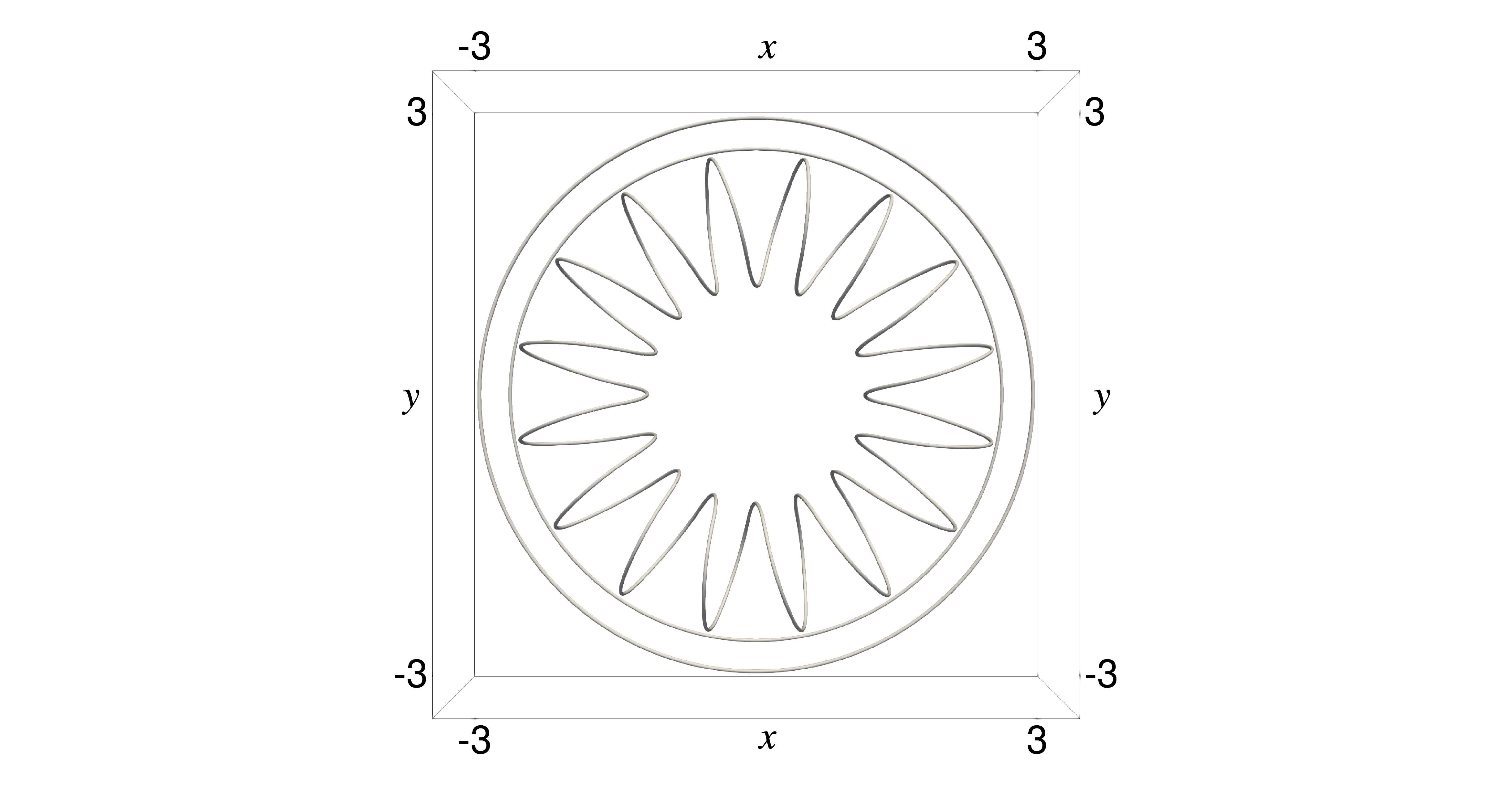
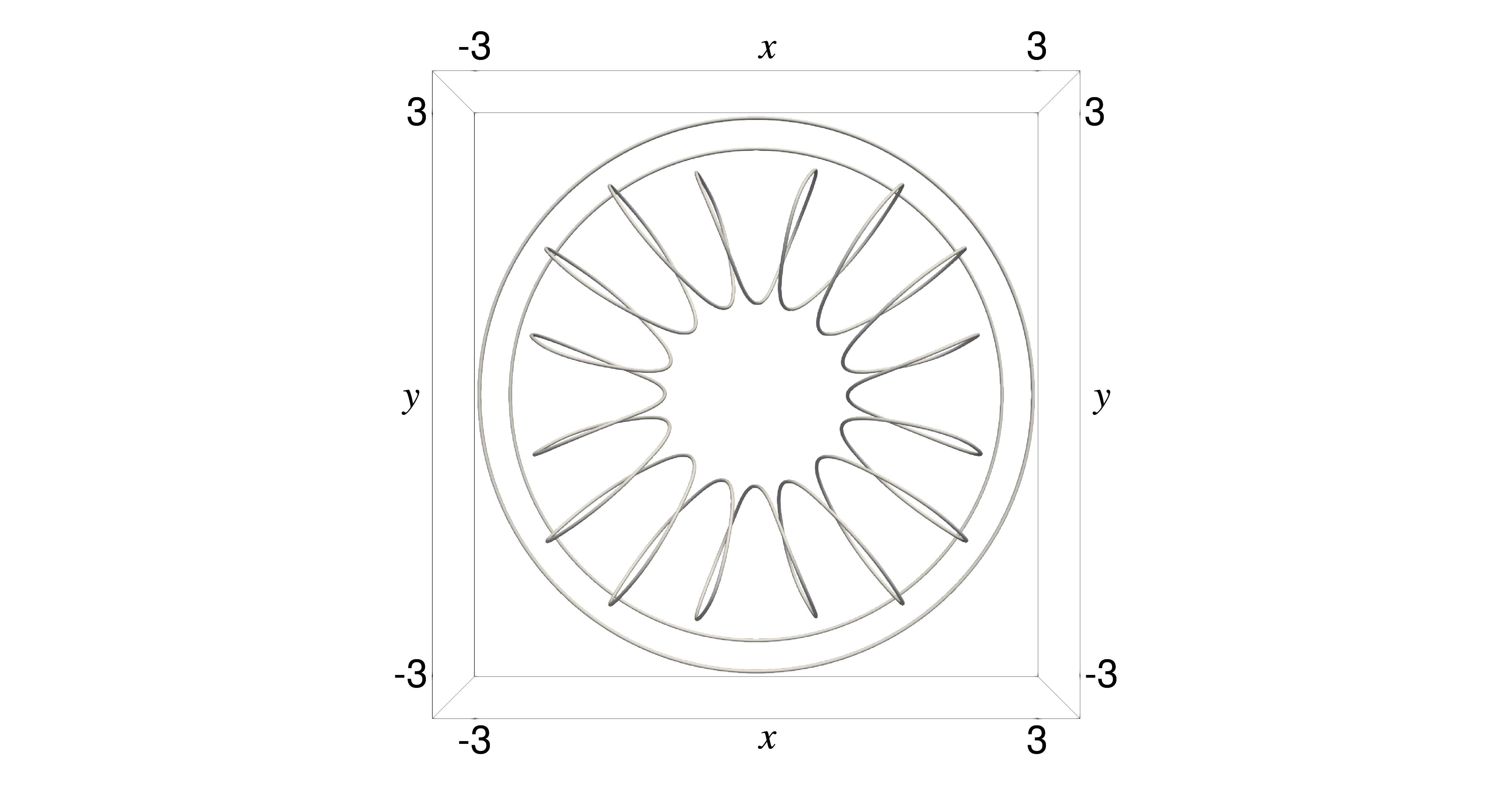
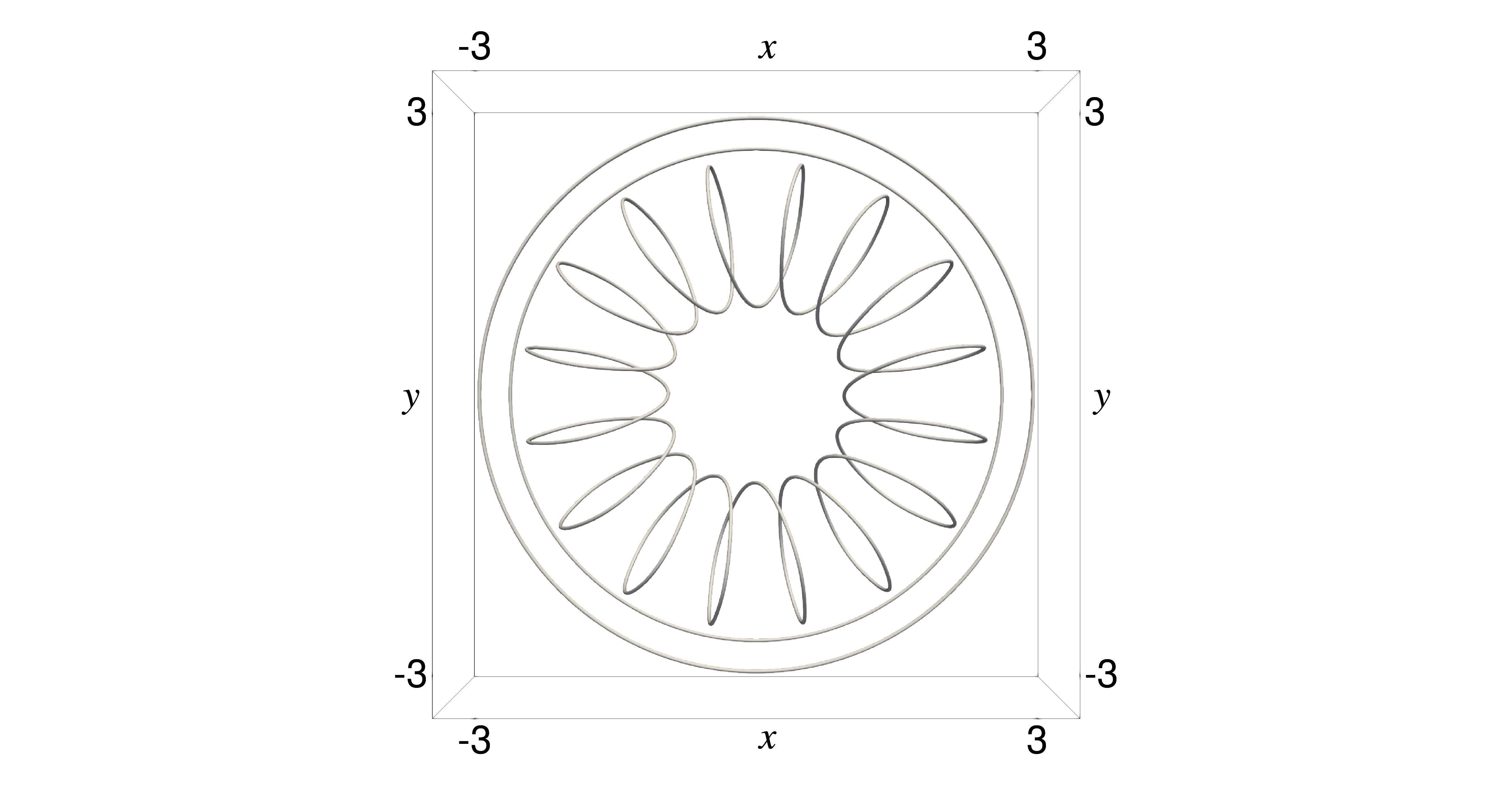
Figure 14 shows the optimised shapes in comparison with the initial shape, which is common to all the cases. It is observed that each turn was deflected in the direction of the magnetic field (i.e., counter-clockwise when viewed from the positive z-axis). Further, the resulting shapes achieved certain symmetries, which are not assumed explicitly. Especially, Case III, where the length of the toroidal coil is constrained, resulted in a rotational symmetry with respect to the z-axis. Meanwhile, Cases I and II obtained a different type of symmetry due to the constraints regarding the coordinates of CPs.
Finally, Figure 15 plots the vector field B on the planes y = 0.0 and z = 0.0. From the result of the former plane, it is observed that the magnetic field was more attracted to the toroidal coil C (1) in Cases II and III. However, the field on z = 0.0 shows that the field inside C (1) was not particularly reinforced or confined by the optimisation even in those cases.
In order to assess the magnetic confinement more precisely, it is necessary to take account of the strength of B inside the toroidal coil into the objective function, according to the previous study [19], for example. 3 The resulting SO is a multi-objective optimisation but out of scope of the present article.
Although the present example is not practical but rather mathematical, it successfully demonstrated the ability of the proposed SO system to handle a large and complicated problem.
This study presents a shape optimisation (SO) framework to achieve desired mutual inductances (MIs) between coils in three-dimensional space by manipulating their geometries. The key theoretical contribution lies in the derivation of the shape derivative of the objective function, defined as the deviation from the target MIs. To accommodate 3 Another idea is to maximise the self-inductance of C (1) . However, such a self-inductance involves a diverging contour-integral and thus unavailable as an objective function in the wire model employed by this study.
17
Figure 13: Example 3: (Left) History of J. (Right) History of the length of the toroidal coil C (1) .
arbitrary coil shapes, the coils are presented by closed B-spline curves, following the approach of Takahashi et al. [19]. Consequently, the shape of each coil can be designed by its control points (CPs). Furthermore, a constraint on the coil length is formulated in terms of these CPs. The resulting SO system enables us to solve an SO problem using a quasi-Newton method, treating the discretised shape derivative as the gradient of the objective function.
In Section 4, numerical experiments were conducted to quantitatively and qualitatively validate the theoretical and numerical developments of the proposed SO system. However, the application of this system to more practical optimisation scenarios, including multi-objective optimisations involving MIs, remains a subject for future investigation.
Acknowledgements
The authors express their gratitude to the anonymous referee for their constructive feedback, which greatly enhanced the quality of this manuscript.
18
Initial shape
19 Data Availability Statement
The software and the associated data that support the findings of this study are available from the corresponding author upon reasonable request.
Declaration of generative AI and AI-assisted technologies in the writing process
During the preparation of this work the authors used Google’s Gemini (2.0 Flash) in order to improve language and readability. After using this tool/service, the authors reviewed and edited the content as needed and take full responsibility for the content of the publication.
References [1] F. Grover, Inductance Calculations: Working Formulas and Tables, Dover phoenix editions, Dover Publications, 2004.
[2] H. Chan, K. Cheng, D. Sutanto, A simplified neumann’s formula for calculation of inductance of spiral coil, 2000, pp. 69–73.
doi:10.1049/cp:20000222. [3] C. L. W. Sonntag, E. A. Lomonova, J. L. Duarte, Implementation of the neumann formula for calculating the mutual in-
ductance between planar pcb inductors, in: 2008 18th International Conference on Electrical Machines, 2008, pp. 1–6. doi:10.1109/ICELMACH.2008.4799978. [4] C. Akyel, S. Babic, M.-M. Mahmoudi, Mutual inductance calculation for non-coaxial circular air coils with parallel axes, Progress In
Electromagnetics Research 91 (2009) 287–301. doi:10.2528/PIER09021907. [5] E. R. Joy, A. Dalal, P. Kumar, Accurate computation of mutual inductance of two air core square coils with lateral and angular misalign-
ments in a flat planar surface, IEEE Transactions on Magnetics 50 (1) (2014) 1–9. doi:10.1109/TMAG.2013.2279130. [6] X. Zhang, H. Meng, B. Wei, S. Wang, Q. Yang, Mutual inductance calculation for coils with misalignment in wireless power transfer, The
Journal of Engineering 2019 (16) (2019) 1041–1044. doi:10.1049/joe.2018.8670. [7] Y. Cheng, Y. Shu, A new analytical calculation of the mutual inductance of the coaxial spiral rectangular coils, IEEE Transactions on
Magnetics 50 (4) (2014) 1–6. doi:10.1109/TMAG.2013.2290972. [8] E. Paese, M. Geier, R. Homrich, R. Rossi, A coupled electric–magnetic numerical procedure for determining the electromagnetic force
from the interaction of thin metal sheets and spiral coils in the electromagnetic forming process, Applied Mathematical Modelling 39 (1) (2015) 309–321. doi:10.1016/j.apm.2014.05.032. [9] Y. Itoh, H. Utoh, Y. Sakamoto, R. Hiwatari, Joint Special Design Team for Fusion DEMO, Empirical formulas for estimat-
ing self and mutual inductances of toroidal field coils and structures, Plasma and Fusion Research 15 (2020) 1405078–1405078. doi:10.1585/pfr.15.1405078. [10] M. Seoane, P. Ledger, A. Gil, M. Mallett, An accurate and efficient three-dimensional high-order finite element methodology for the
simulation of magneto-mechanical coupling in MRI scanners, International Journal for Numerical Methods in Engineering 119 (12) (2019) 1185–1215. doi:10.1002/nme.6088. [11] M. S. Miah, P. D. Ledger, A. J. Gil, M. Mallett, T.-Q. Ye, An application of hp-version finite element methods to quench simulation in
axisymmetric MRI magnets, Engineering with Computers (2025). doi:10.1007/s00366-025-02126-y. [12] L. Tian, L. Song, Y. Zheng, J. Wang, Design and evaluation of magnetic field strength detection devices for millimeter-sized planar square
inductors based on a mutual coupling model, Review of Scientific Instruments 93 (9) (2022) 094102. doi:10.1063/5.0075990. [13] A. Yadav, T. K. Bera, Design and optimization of circular and rectangular couplers for wireless power transfer: efficiency enhancement and
human safety assessment 5 (2 2025). doi:10.1007/s43937-025-00065-9. [14] M. Kiani, U.-M. Jow, M. Ghovanloo, Design and optimization of a 3-coil inductive link for efficient wireless power transmission, IEEE
Transactions on Biomedical Circuits and Systems 5 (6) (2011) 579–591. doi:10.1109/TBCAS.2011.2158431. [15] Z. Duan, Y.-X. Guo, D.-L. Kwong, Rectangular coils optimization for wireless power transmission, Radio Science 47 (3) (2012).
doi:10.1029/2011RS004970. [16] K. Krestovnikov, E. Cherskikh, B. Aleksandr, Approach to choose of optimal number of turns in planar spiral coils for systems of wireless
power transmission, Elektronika ir Elektrotechnika 26 (6) (2020) 17–24. doi:10.5755/j01.eie.26.6.26181. [17] Y. Ben Fadhel, G. Bouattour, D. Bouchaala, N. Derbel, O. Kanoun, Model-based optimization of spiral coils for improving wireless power
transfer, Energies 16 (19) (2023). doi:10.3390/en16196886. [18] S. Hurwitz, M. Landreman, P. Huslage, A. Kaptanoglu, Electromagnetic coil optimization for reduced lorentz forces, Nuclear Fusion 65 (5)
(2025) 056044. doi:10.1088/1741-4326/adc9bf. [19] T. Takahashi, Designing gradient coils with the shape derivative and the closed b-spline curves, Magnetic Resonance Imaging 110 (2024)
112–127. doi:10.1016/j.mri.2024.03.042. [20] J. D. Jackson, Classical Electrodynamics, 3rd Edition, Wiley, New York, NY, 1999. [21] S. G. Johnson, The NLopt nonlinear-optimization package, http://github.com/stevengj/nlopt.
URL http://github.com/stevengj/nlopt [22] M. Abramowitz, I. Stegun (Eds.), Handbook of Mathematical Functions: with Formulas, Graphs, and Mathematical Tables (eighth Dover
printing), Dover, New York, 1972.
20 Initial shape 4 1.0 4
3
0.8 1 1
y |B| 0.6
0
0.4 -1
-2 0.8 2 0.6
|B| 2 z 1.0
3 0
0.4 -1
-2 0.2 -3 0.2 -3
-4 0.0
-4 -3 -2 -1 0
x1 2 3 -4 4 0.0 -4 -3 -2 -1 0
x1 2 3 4 Optimised shape (Case I) 4 1.0 4
3 3
0.8 1 1
y |B| 0.6
0
0.4 -1
-2 0.8 2 0.6
|B| 2 z 1.0 0
0.4 -1
-2 0.2 -3 0.2 -3
-4 0.0
-4 -3 -2 -1 0
x1 2 3 -4 4 0.0 -4 -3 -2 -1 0
x1 2 3 4 Optimised shape (Case II) 4 1.0 4
3
0.8 1 1
y |B| 0.6
0
0.4 -1
-2 0.8 2 0.6
|B| 2 z 1.0
3 0
0.4 -1
-2 0.2 -3 0.2 -3
-4 0.0
-4 -3 -2 -1 0
x1 2 3 -4 4 0.0 -4 -3 -2 -1 0
x1 2 3 4 Optimised shape (Case III) 4 1.0 4
3
0.8 1 1
y |B| 0.6
0
0.4 -1
-2 0.8 2 0.6
|B| 2 z 1.0
3 0
0.4 -1
-2 0.2 -3 0.2 -3
-4 0.0
-4 -3 -2 -1 0
x1 2 3 -4 4 0.0 -4 -3 -2 -1 0
x1 2 3 4 Figure 15: Example 3: Distribution of the magnetostatic field B on the plane y = 0.0 (left) and z = 0.0 (right). The maximum of |B| is truncated to 1.0. 21