⬇ Download Markdown · ⬇ Download LaTeX · ⬇ original · view original · CSV: table 1
Magnetic-field-tuned randomness in inhomogeneous altermagnets
Anzumaan R. Chakraborty, 1, 2 Jörg Schmalian, 3, 4 and Rafael M. Fernandes 1, 2
1 Department of Physics, The Grainger College of Engineering, University of Illinois Urbana-Champaign, Urbana, IL 61801, USA 2 Anthony J. Leggett Institute for Condensed Matter Theory, The Grainger College of Engineering,
University of Illinois Urbana-Champaign, Urbana, 61801, IL, USA 3 Institute for Theory of Condensed Matter, Karlsruhe Institute of Technology, 76131 Karlsruhe, Germany
4 Institute for Quantum Materials and Technologies, Karlsruhe Institute of Technology, 76126 Karlsruhe, Germany
(Dated: July 18, 2025)
Altermagnetic (AM) states have compensated collinear magnetic configurations that are invariant under a combination of real-space rotation and time reversal. While these symmetries forbid a direct bilinear coupling of the AM order parameter with a magnetic field, they generally enable piezomagnetism, manifested as a trilinear coupling with magnetic field and strain. Here, we show that, because of this coupling, in an altermagnet subjected to random strain, the magnetic field triggers an effective random field conjugate to the AM order parameter, providing a rare realization of a tunable random-field Ising model. Specifically, we find two competing effects promoted by an external magnetic field: an increasing random-field disorder, which suppresses long-range AM order, and an enhanced coupling to elastic fluctuations, which favors AM order. By solving the corresponding random-field transverse-field Ising model via a mean-field approach, we obtain the temperature-magnetic field phase diagram of an inhomogeneous AM state for different strengths of random-strain disorder, unveiling the emergence of a field-induced reentrant AM phase. We also discuss the fingerprints of this rich behavior on several experimentally-accessible quantities, such as the shear modulus, the elasto-caloric effect coefficient, and the AM order parameter. Our results reveal an unusual but experimentally-feasible path to tune AM order with uniform magnetic fields.
A recent classification of collinear magnetism revealed the existence of three different types of magnetic states: ferromagnetism, antiferromagnetism, and altermagnetism [1–3]. These different magnetic ground states, which are formally defined in the absence of spin-orbit coupling using the concept of spin groups [3–7], are distinguished according to the type of space group operation which, when combined with time-reversal, leaves the ground state invariant. In ferromagnets (FM), there is no such operation and a uniform splitting between spinup and spin-down bands emerges. Time-reversed antiferromagnetic (AFM) ground states, on the other hand, are related by a translation or inversion, resulting in a symmetry-protected Kramers spin degeneracy throughout the entire Brillouin zone. Finally, time-reversed altermagnetic (AM) ground states are related by any crystalline operation that is not translation or inversion, such as rotation, mirror reflection, or non-symmorphic operations like glides or screw rotations. The implication of
split band structure, with spin degeneracy preserved only along certain high-symmetry momentum space planes (for a recent review, see [8]). These unusual properties have motivated extensive theoretical works on the interplay between altermagnetism and other electronic phenomena such as topology [9–16], electronic correlations [17–23], superconductivity [24–38], non-trivial responses [39–48], and multiferroics [49–51].
Many materials have been proposed to realize altermagnetism, from metals to Mott insulators [52– 61]. Among those, experiments have directly demonstrated the altermagnetic character of materials such as MnTe [62–65], CrSb [66–69], Co 1/4 NbSe 2 [70–72], and AV 2 Ch 2 O (with alkali metal A = Rb, K and chalcogen Ch = Se, Te) [73], while results for RuO 2 remain under debate [74–82]. More broadly, altermagnetism is connected to other problems of interest in condensed matter physics beyond spin-splitting in compensated magnets [83–86]. For example, altermagetic order breaks the same symmetries as other states of interest in correlated electron systems, such as ferro-octupolar order [10, 42, 87] in multipolar magnets [88–91] and metals undergoing an even-parity spin-triplet Pomeranchuk instability [92–94]. The microscopic mechanisms involved, however, are very different, as the crystalline potential plays an essential role in stabilizing altermagnetism [95]. Thus, given the rich landscape of materials and phenomena related to altermagnetism, it is important to establish which external perturbations can be used to control and probe these systems.
At first sight, one may think that a magnetic field H is not an ideal tuning parameter for altermagnetism. Indeed, since H cannot couple directly (i.e., via a bilinear coupling) to the AM order parameter Φ(x), one would expect H to have a minimal effect on the onset of AM order. However, the symmetries that define altermagnetism also imply that nearly all altermagnets display piezomagnetism [10, 40, 43, 96, 97]. Piezomagnetism is a 2
3 cient, thus providing concrete experimental predictions to verify this behavior in candidate AM materials.
This paper is organized as follows. In Sec. II we construct an effective random-field transverse-field Ising model (RF-TFIM) for an AM system [110]. This model consists of a uniform transverse field Γ encapsulating the role of quantum fluctuations, and a longitudinal field H z that promotes the coupling between Φ and shear strain ε. We compute the mean-field phase diagram of this model as a function of the parameters T, Γ, H z , and intrinsic random strain. In Sec. III we compute the order parameter self-consistently and obtain the AM susceptibility, shear modulus renormalization, and elasto-caloric effect both as a function of T and of H z . Like in the case a nematic critical point, we find a softening of the shear modulus at the AM critical point signaling an accompanying structural transition. In Sec. IV, we discuss the effect of fluctuations beyond mean-field, which are typical for random field models without infinite-range interactions. Finally, we present our conclusions in Sec. V, and in the Appendix, we provide additional details of the calculation for the elasto-caloric effect coefficient.
UNIFORM TRANSVERSE FIELD For concreteness, we consider a specific d-wave AM ordered state in the tetragonal lattice (with point group D 4h ) that displays piezomagnetism. In the presence of SOC, the components of the vector AM order parameter Φ transform as different irreducible representations (irreps) of the point group according to the direction of the magnetic moments. For out-of-plane moments, the system remains a “pure” altermagnet even in the presence of SOC [10], and the AM order parameter Φ is Ising− like, transforming either as the B
1g irrep (in the case
AM, as relevant for La 2 Mn 2 Se 2 O 3 [61] and AV 2 Ch 2 O [59, 60, 73, 111]). Here, the minus superscript indicates that the irrep is odd under time-reversal symmetry. Us-
straightforward to derive Eq. (2) and obtain the Landau free-energy invariant [40]:
where λ is the piezomagnetic coupling, ε ≡ ε xy in the case of a d xy -wave AM and ε ≡ ε x 2 −y 2 in the case of a
To proceed, we write down an effective low-energy model for the coupled AM-strain degrees of freedom. As explained above, for a tetragonal lattice, the d-wave
parameter (Φ above). To account for the role of spatial and quantum fluctuations, we promote this homogeneous order parameter to a coarse-grained local Ising (i.e., pseudo-spin) variable τ i z , such that ⟨τ i z ⟩ = Φ. Spatial fluctuations are encoded in the effective interaction between the pseudo-spins, whereas quantum fluctuations appear as a transverse field to the pseudo-spin. Thus, our phenomenological Hamiltonian for the AM phase is that of a transverse-field Ising model:
where, as discussed above, τ i z and τ i x are Pauli matrices. J is an effective AM interaction, whose origin depends on the microscopic mechanism behind AM order, that sets the scale of the thermal AM transition (and should not be confused with an exchange interaction). The transverse field Γ is a non-thermal parameter (such as doping or pressure) that promotes quantum fluctuations, i.e., tunneling between local pseudo-spin states. Thus, as Γ is enhanced, the ordered state is suppressed and the system is driven to a quantum critical point (QCP). Note that, being phenomenological, our approach is agnostic about the microscopic origin of the AM order parameter. For instance, in the Lieb lattice model of Ref. [12], τ i z could correspond to the staggered magnetization between the two sublattices related by a 90 ◦ rotation, coarse-grained over a single square plaquette. It could also correspond to the average magnetic octupole moment on the third site of the Lieb lattice, or to some combination of them [43] determined by the energetics of the microscopic model [87]. The key point is that, regardless of the microscopic mechanism, the AM ordered state will occur due to the condensation of an Ising-like order parameter that transforms as the appropriate irrep.
Strain fields in crystals are usually inhomogeneous, ε → ε(x), with two contributions arising from distinct phenomena. The first is a non-singular contribution from thermally excited elastic fluctuations ε 0 (q), associated
AM. The second is a singular contribution from random strain arising from crystal defects ε s (x) in the form of a quenched random field. Therefore, from Eq. (3), we can cast the inhomogeneous piezomagnetic term as:
Note that the elastic fluctuations are well-defined excitations; therefore ε 0,i should be thought of as an annealed dynamical field which one can integrate out. The effect of the non-homogeneous part of ε 0,i , i.e., the q ̸ = 0 modes, is to drive the AM transition mean field and renormalize the effective Hamiltonian [112, 113]. We therefore 4 dispense with ε 0 (q ̸ = 0) modes and regard them as subleading corrections to the full Hamiltonian. By contrast, ε s,i represents quenched disorder and remains as a fixed realization of a random field drawn from a zero-mean probability distribution. Putting it all together, the effective Hamiltonian consisting of altermagnetic and elastic degrees of freedom is
where N denotes the number of sites.
III.
A.
FIELD-TUNED ALTERMAGNETIC
TRANSITION and further justify replacing the original nearest-neighbor interaction with an all-to-all interaction.
The second term of H̃ describes the contribution to the piezomagnetic coupling due to random strain, with the product λH z ε s,i taking the role of an effective random longitudinal field conjugate to the AM order parameter. Given that an infinite-range interaction, a random field, and a non-random transverse field are present,
Ising model (RF-TFIM) [110, 114]. Including dynamical phonons changes the infinite-range coupling to a dipolar interaction, an effect that we ignore in our subsequent analysis.
We now make a few convenient substitutions. First, we express all energy scales in units of J by setting J = 1. Second, we express the Hamiltonian in a dimensionless
H̃/ J ˜ = − Renormalized field-dependent Hamiltonian In this section, we analyze the phase diagram of Eq. (6) within mean-field over a wide range of parameters, including the strength of quantum fluctuations, temperature, disorder strength, and magnetic field. To formally perform a mean-field calculation, we extend the AM interaction J to also be infinite-range rather than nearestneighbors:
Here
is a dimensionless quantity that gives the elastic energy of the random distribution of strain in units of the AM interaction J. In what follows, the standard deviation of the random variables W shall be regarded as a parameter of the problem. Similarly, the temperature and 5 transverse field in these dimensionless units are
where, we recall, T and Γ are given in units of J.
To set the stage, we provide a qualitative description of the phase diagram in the four-dimensional (h, W, Γ, T ) parameter space. In the classical limit Γ = 0, Eq. (12) describes the well-known infinite-range RFIM, for which there exists a critical random field strength w c separating an ordered and a disordered phase [102]. Unlike the prototypical RFIM, however, here the random field strength w(h) is tunable by magnetic field, suggesting the possibility of field values h 1 and h 2 for which w(h 1 ) < w c
the ordered and disordered phases. Additionally, w(h) is non-monotonic, and reaches a maximum value of W ∝ ε̄ s at h = 1. Therefore three possibilities exist when the system begins in the ordered phase and a magnetic field is applied, which we delineate as follows:
• In the regime of strong disorder, W exceeds w c .
The non-monotonicity of w(h) implies the existence
plies the phenomenon of altermagnetic reentrance, in which the AM order parameter Φ is nonzero for
• In the regime of weak disorder, W is smaller than
w c . As a result, the system remains trapped in the ordered phase. Interestingly, the order parameter Φ exhibits a vestige of the reentrance behavior characteristic of the strong disorder case, as it attains a non-zero minimum value Φ min at a field value h min < 1 for arbitrarily small W ∝ ε̄ s . • In the marginal disorder regime, W = w c . As a
result, w(h) = w c exhibits a double root h = h ∗ . Given that h ∗ is a double root, tuning the magnetic field across h ∗ amounts to running tangent to the co-dimension 1 phase boundary at precisely
deform with Φ min going to zero at a single point h ∗ . This gives rise to a “V”-like behavior of the order parameter, Φ ∝ |h − h ∗ |. This unusual phenomenon, which we explore in Section III, reflects the nontrivial RF-TFIM parameter space enabled by the piezomagnetic coupling. The presence of thermal and quantum fluctuations reduces the critical strength w c , i.e., increases the effec-
tive disorder. Formally, this means that the function w c (Γ, T ) decreases with increasing Γ and T , and consequently, the reentrant behavior is enhanced, as the para-
an intrinsic property of the crystal, it is unlikely to be tunable. Therefore, to assess the features of the phase diagram delineated above one must tune Γ and T so that the function w c (Γ, T ) becomes greater than, equal to, or less than the intrinsic random strain scale W .
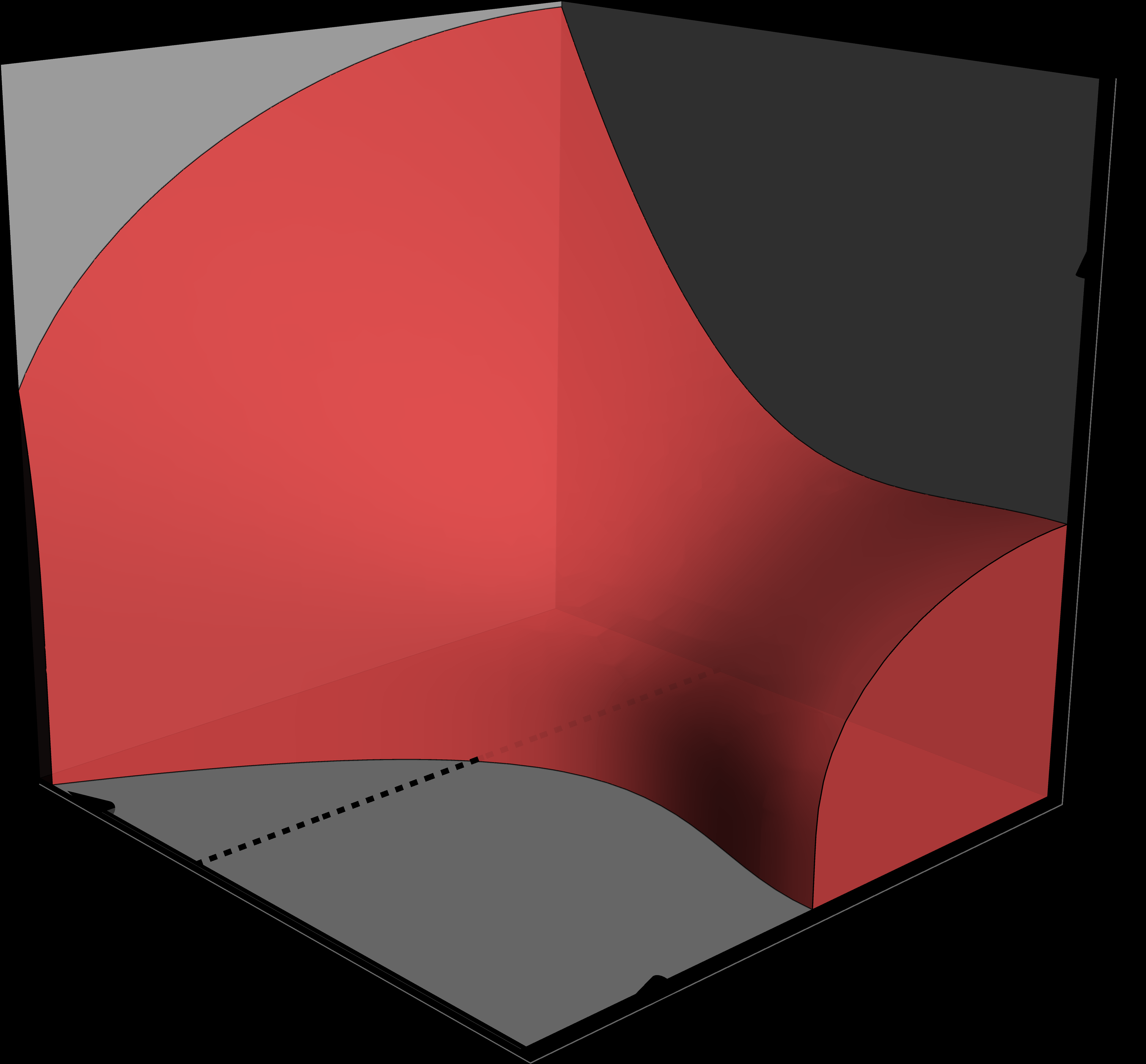
We now construct the mean-field T = 0 phase diagram of Eq. (8) as a function of h, Γ, and W , which is shown in Fig. 2. In preparation for the finite temperature case, for which there are four parameters (h, W, Γ, T ) rather than three, we describe two complementary approaches to visualize the phase diagram. The first is to construct
and γ(h), where the AM-PM phase boundary appears as a convex curve bounding the origin (Fig. 3a). Tuning h
tory in this (w, γ)-plane, which may or may not intersect with the phase boundary depending on the values of W and Γ. The second approach is to construct multiple 2D phase diagrams, one for each W – corresponding to different strengths of random strain – with h and Γ as dimensionless axes (Fig. 3b-e). In this case, tuning away 6
t
sets the starting point of the phase trajectory along the γ-axis and W (listed in the legend) sets the maximum extent of the trajectories along the w-axis. Increasing the magnetic field moves the system along the trajectory as indicated by the
respectively. As the disorder strength W increases, the paramagnetic region grows and the AM-PM transition line forms a
from the h = 0 limit amounts to following a line parallel to the h-axis. The appearance of reentrance over some parameter regime manifests as a “bulge” in the AM-PM phase boundary. Finally, a third, which is relevant only for the T = 0 case, is to represent the full (h, W, Γ) phase diagram, as depicted in Fig. 2.
We delineate the first approach now. The hparameterized trajectory θ in this (w, γ)-plane is given by
(19)
(20)
When h = 0, the effective coupling between Φ and random strain vanishes, leading to no renormalization of γ, so γ(h) = Γ. When h = 1, the effective random field width w(h) reaches its maximum value of W . Finally, as h → ∞ the enhanced interaction suppresses γ and w and the order parameter saturates to unity in the fully ordered state corresponding to w = γ = t = 0.
Appropriate for the case of infinite-range interactions, we solve the RF-TFIM of Eq. (12) at T ≥ 0, following
tonian
bers a and b, and we assume each disorder realization {z i } to consist of independent and identically distributed Gaussian random variables drawn from the distribution
7 For each disorder realization, we compute the dimension-
T log Z[z i ] less free energy density f = − ˜ JN
(23) Assuming replica symmetry, we subsequently disorder-
In Eq. (24), we have defined the non-negative function Λ(z) which encapsulates all of the t(h) and γ(h) dependence of the problem
By expanding the integrand in powers of Φ, the quadratic and quartic Landau coefficients can be written compactly as
Since p(z) is Gaussian and since Λ(z) grows algebraically, total derivative terms vanish. Consequently, one can “trade” z derivatives between p(z) and Λ(z) at will using integration-by-parts. In the limit of zero temperature, Λ simplifies dramatically:
Analytical expressions for the quadratic and quartic coefficients can be expressed using special functions:
where
and U (a, b, z) is a confluent hypergeometric function of the second kind, whereas K n (x) is a modified Bessel function of order n. Since U is strictly positive whenever A ≥ 0, the transition between AM and PM phases is second-order. Therefore, vanishing of the quadratic Landau coefficient A = 0 gives the phase boundary.
In the case of the classical RFIM with Γ = 0 the quadratic Landau coefficient takes the form
By solving A = 0 for w, we find the well-known result [102] for the critical disorder strength
When W > W 0 , AM reentrance occurs via a paramagnetic phase bounded by two field values given by
For the case of nonzero Γ, the equation for the phase boundary A = 0 yields a critical disorder strength that decreases monotonically with Γ. We solve this equation and obtain the function w c (γ, t) restricted to the t = 0 plane, i.e., w c (γ, 0). We give the asymptotic behaviors near the clean QCP and classical disorder-induced transitions, respectively:
For fixed Γ, we may also obtain the minimum W required to achieve reentrance. This minimum W , which we call
Solving these two equations yields W ∗ and the magnetic
as an identity through the functional equation
(38)
We plot W ∗ (Γ) and h ∗ (Γ) in Fig. 4a-b, showing that the threshold disorder strength W ∗ (Γ) and threshold field h ∗ (Γ) fall monotonically with increasing Γ. The values at the classical limit Γ = 0 and at the QCP Γ = 1 are, respectively
8
This implies that from the definition of W , reentrance requires the energy scale of the random strain E el = 2 1 C 0 ε̄ 2 s to be of order J even at the QCP, where quantum disordering effects are the strongest. Conversely, the magnetic fields at which reentrance occurs are suppressed rapidly close to the QCP because h ∗ → 0 as Γ → 1.
Figure 4. (a) Threshold disorder strength W ∗ /W 0 and (b) corresponding magnetic field value h ∗ as functions of
remains of order one, whereas h ∗ vanishes rapidly. This means that AM reentrance and order parameter non-monotonicity as a function of h are favored when starting close to the zero magnetic field critical point.
The key advantage of representing the zero temperature phase diagram in the scaled coordinates γ and w, as in Fig. 3(a), is that it does not explicitly depend on W and Γ and only does so implicitly through w(h) and γ(h). The drawback is that different W correspond to differently curved phase trajectories θ. Thus, this representation may not be the most obvious physically motivated one and could obscure global features of the AMPM phase boundary without a direct quantitative calculation. In some cases, it is more revealing to construct the zero-temperature phase diagram in coordinates for which the experimentally tunable quantity h appears as an independent axis. This ensures that tuning magnetic field amounts to following a straight line, rather than a curve, for a fixed value of Γ and W , with the drawback being that the phase boundary in these new coordinates depends explicitly on W .
We plot these (Γ, h) phase diagrams for increasing val-
Figure 5. Mean-field TFIM phase diagram, corresponding to W = 0 in our case, plotted against scaled axes t ≡ T /(1 +
t c = γ/ tanh −1 γ decreases with increasing γ, vanishing at a quantum critical point at γ = 1 (in green). Increasing h ≡ H z /H λ amounts to following a straight-line trajectory from
monotonically due to the coupling to elastic fluctuations but no coupling to random strain.
ues of fixed W in Fig. 3(b)-(e). In panels (b) and (c), W < W 0 , implying that the phenomenon of reentrant AM does not occur in the classical regime of Γ = 0. Nevertheless, there is an important distinction between these two cases: in panel (b), because W < W ∗ min < W 0 ,
this case, all that the magnetic field can do is tune the system from the PM to the AM phase, but it cannot tune the AM transition to zero. In contrast, in panel (c), W ∗ min < W < W 0 , and the PM-AM phase boundary shows a “bulge” signaling a reentrant AM phase. This
and moves rapidly upward and to the left as W in-
(d), the tip of the bulge annihilates at the Γ = 0 axis, resulting in a non-analytic behavior of the free energy, as we discuss in Section IV. Finally, when W > W 0 , illustrated in panel (e), reentrance occurs across the entire phase diagram between the critical fields h ± c satisfying Eq. (35). The combination of these panels gives the schematic three-dimensional phase diagram of Fig. 2.
We now construct the finite temperature phase diagram in the four dimensional parameter space spanned 9
paramagnet m alter alt er paramagnet altermagnet t agne altermagnet paramagnet ma gn
et
sets the starting point of the phase trajectory along the t-axis and W sets the maximum extent of the trajectory along the w-axis. Green and blue curves correspond to W = 0.9W 0 and W = 1.05W 0 , respectively. Panels (b) and (c) show the phase diagrams with unscaled axes h = H z /H λ and T corresponding to W = 0.9W 0 and 1.05W 0 , respectively. As the relative disorder W is increased, the paramagnetic region
grows via the formation of a bulge in the AM-PM transition line at (T ∗ , h ∗ ), which
by (h, W, Γ, T ). As with the T = 0 case, we represent the phase diagram in two different coordinate systems. The first is a 3D phase diagram with h-dependent coordinates (w, γ, t), where a changing magnetic field amounts to following a trajectory Θ(h) in this space:
As in the case of zero temperature, W represents the maximum extent of this trajectory along the w-axis.
Before going further, we consider two limiting cases for T ≥ 0: the pure transverse field Ising model TFIM with W = 0 and the classical RFIM with Γ = 0. In both cases, T c decreases monotonically with increasing Γ and W , resulting in QCPs at Γ = 1 and W = W 0 , respectively. These two QCPs are connected by a line of QCPs (Fig. 3a) whose shape on the (Γ, W )-plane depends on h.
When treating the pure TFIM, p(z i ) in Eq. (22) becomes a delta function, and the equation A = 0 for the phase boundary simplifies to
This yields the equation on T c :
(43)
In this case without disorder, Φ couples only to elastic fluctuations, and increasing the magnetic field can only further order the system. This agrees with Eq. (43), from which we see that increasing h suppresses the denominator and enhances T c . The TFIM phase diagram represented in the (t, γ)-plane gives a convex curve – shown in
a straight line connecting the initial point to the origin:
Therefore, in the clean case, the magnetic field can be used to tune the system from the PM phase to the AM phase, but not the other way around.
We now consider the classical RFIM case, for which Γ = 0. In this limit, Λ(z) simplifies, such that A = 0 gives
Solving for w yields the function w c (γ, t) along the γ = 0 plane which has asymptotic behaviors given by
Temperature and transverse field take qualitatively the same role. Both suppress Φ and both are renormalized in the same way due to elastic fluctuations. Therefore, 10
In Fig. 7, we plot the critical surface in these scaled coordinates and show several phase trajectories. As with the previous section, we also display the critical surface in the (h, Γ, T ) parameter space for different values of W . In Fig. 8, we see that when
the single altermagnetic phase region separates at
gions, one at low fields h < 1 and one at high fields h > 1. In this W regime, altermagnetic reentrance is guaranteed to occur even at T = 0. (51)
IV. This yields the threshold values W ∗ and h ∗ as functions of Γ and T , which, at finite temperatures, have a qualitatively similar behavior than the T = 0 case shown in Fig. 4. We note that W ∗ (Γ, T ) remains of order one and is never suppressed to zero, suggesting that E el must be of order J for reentrance to occur, like in the zero temperature case. However, we stress that h ∗ can be made arbitrarily small depending on how close (Γ, T ) is to the transition when H z = 0. Generalizing from the two-dimensional cases, h ∗ (Γ, T ) and W ∗ (Γ, T ) are related through the functional equation
(53)
(52)
EXPERIMENTAL SIGNATURES The phase diagrams shown in Fig. 8 reveal that, in an inhomogeneous altermagnet, application of a magnetic field can induce both a PM-AM transition, when the disorder strength is weak, as well as an AM-PM-AM transition with reentrant altermagnetic order, when the disorder strength is strong. In this section, we go beyond the determination of the phase transition boundaries and discuss the behavior of three experimentally observable quantities as the phase boundaries are traversed by a magnetic field: the altermagnetic order parameter, the shear modulus, and the elasto-caloric effect coefficient. Note that, in principle, the AM order parameter could be measured in momentum space from the spin splitting of 11
the band structure, or from extracting response functions that are proportional to the order parameter, such as the piezomagnetic and the elasto-Hall conductivity tensors [47].
We first consider (Γ, T ) values that place the system inside the AM ordered phase in the absence of a magnetic field. We also specialize to the case of W < w c (Γ, T ) for which long-range AM order remains intact for all values of h. Although an AM reentrant behavior does not take place, we show that Φ(h) displays a non-monotonic behavior and a minimum value Φ min for h = h min .
The mean field equation ∂ f ¯ /∂Φ = 0 gives a selfconsistent condition for the order parameter:
where we recall that p(z) is a normal distribution with
nonzero Φ satisfies the equation
than unity due to the concavity of the hyperbolic tangent function. Conversely, the limit h → ∞ yields a maxi-
case, the self-consistent equation simply yields |Φ| = 1, i.e., the order parameter saturates to its maximum value.
small h, increasing h amounts to merely increasing the effective random field width w, which can only suppress Φ. These three facts together, namely that Φ(h = 0) ≤ 1,
establishes that Φ must have a minimum at some magnetic field value h = h min . It is straightforward to conclude that h min must be less than 1, because an upturn in Φ can only happen when a nontrivial competition between the ordering and disordering tendencies occurs, i.e., when the effective energy scales w(h), γ(h), and t(h) are not all decreasing, which can only happen if h < 1. Generally, we can then write
where the combination of the self-consistent equation and the condition dΦ/dh = 0 yields a system of equa-
Φ min (W, Γ, T ). We stress, however, that in the case of Φ = O(1) deep inside the ordered phase, the necessity of minimizing the infinite-order expression for f ¯ (Φ) yields
In light of this fact, it is convenient to focus on the case where the parameter values place the system close to the AM-PM phase boundary, where f ¯ may be truncated to quartic order in Φ. To proceed, we consider phase diagrams like those of Fig. 8(a)-(b), corresponding to W < W 0 (weak disorder). In these cases, reentrant behavior as a function of h can be obtained by tuning the value of Γ. For concreteness, we focus on the T = 0 cut of the phase diagram in the vicinity of the point (Γ ∗ , h ∗ ) that marks the end of the bulge of the PM-AM phase boundary, as shown in the inset of Fig. 9.
al To obtain the form of Φ(h) as the PM-AM phase boundary is traversed upon increasing Γ, we use the phenomenological Landau coefficients. Since Φ is small, we can approximate U to be a constant and equal to U 0 = U(h = h min ). Then, because A is analytic in h and closest to zero when h = h min , we have the approximation t 12 Note that, in the last step, we renamed h min to h ∗ in accordance with the notation of Sec. III. These two behaviors for Φ(h), corresponding to a quadratic minimum and to a cusp are illustrated by the green and blue lines in Fig. 9 .
Figure 9. The AM order parameter Φ plotted as a func-
(red), where Γ ∗ ≈ 0.526. The associated phase diagram (inset) shows the corresponding line cuts in the magnified T = 0 plane. For Γ < Γ ∗ , the order parameter displays an analytic local minimum at h = h min , crossing over between quadratic (near h min ) and linear (away from h min ) regimes. For Γ = Γ ∗ , h min approaches h ∗ ≈ 0.842 at which point Φ vanishes, and the quadratic regime is suppressed completely. For Γ > Γ ∗ , Φ
Upon increasing Γ further, the PM-AM phase boundary is intersected twice at the two critical fields h ± c , signaling the loss of long-range order over a finite range
tory Θ(h) has a nonzero component normal to the phase boundary, and hence the distance to the critical surface scales linearly with |h − h ± c |. For Φ(h), this translates to a “splitting” of the cusp at h ∗ into two successive square+ root singularities at h −
c and h c . We use our Landau theory to investigate what happens + within the ordered phase when h −
c and h c are sufficiently close together. Within the ordered phase, but near h ± c , we obtain for the quadratic coefficient
a crossover regime governed by
that distinguishes between square-root and linear behaviors:
This behavior is illustrated by the red line in Fig. 9. We can also decrease Γ to move back from the reentrant to 13
AM
PM PM PM AM AM
AM
Figure 10. The zero-temperature mean-field order parameter as a function of h = H z /H λ for different values of Γ given in the
panels (a), (b), and (c), respectively. For weak disorder, the order parameter behaves non-monotonically, whereas for strong disorder it exhibits reentrance.
the tangent case. The corresponding limit is h ± c → h ∗ and h ′ t → 0, for which the square-root behavior vanishes and only the cusp-like behavior of Eq. (63) remains. We note that Eq. (66) is an approximation, and higher-order corrections in h ′ t will lead to square-root prefactors that are different for the two critical fields.
While the analysis here focused on the T = 0 phase diagram with weak disorder (W < W 0 ), similar behaviors for Φ(h) are carried over to the phase diagrams of the marginal disorder (W = W 0 ) and strong disorder (W > W 0 ) cases. As shown in Fig. 10, in the former, Φ(h) displays the cusp-behavior for Γ = 0 whereas, in the latter, Φ(h) always shows the square-root-like behavior for any Γ value.
While in the previous section we focused on the behavior of the AM order parameter, in this and in the next subsection we focus on the behavior of the AM susceptibility. The key point is that piezomagnetism enables a coupling between altermagnetic and elastic degrees of freedom such that their fluctuations also become correlated. Consequently, order parameter fluctuations, which become pronounced near the AM transition, enhance elastic fluctuations and lead to a structural transition which accompanies the AM critical point (see also [116]). The situation is analogous to a nematic transition softening the shear modulus [117]. A straightforward mean field calculation of the renormalized shear modulus
where χ is the AM static susceptibility. As expected, the H z = 0 limit results in no renormalization since the effective bilinear strain-AM coupling is zero, whereas H z ̸ = 0 results in the vanishing of the shear modulus at the AM transition where χ → ∞. Using the definition of H λ , Eq. (67) can be written in a dimensionless fashion:
This analysis reveals a clear analogy between nematicity and altermagnetism [116]. In nematicity, a direct bilinear coupling between the order parameter and shear strain is symmetry-allowed, resulting in a structural distortion at the nematic transition. This coupling of an electronic order parameter to the lattice, and subsequent structural distortion, is a key ingredient in the elucidation of nematicity in correlated systems [118, 119]. By contrast, in the altermagnetic case, this effective coupling and the resulting structural distortion magnitude is tunable by a magnetic field.
To calculate the renormalized shear modulus, we use our Landau theory to ascertain χ in both the PM and AM phases. In mean field theory, χ exhibits Curie-Weiss-like universal behavior proximate to the phase boundary in 14 new free energy which
To lowest order in B, the saddle-point equation ∂ Φ f ¯ B = 0 can be written as PM AM
where only the B = 0 free energy f ¯ , defined in Eq. (24), is invoked. Differentiating Eq. (72) with respect to b and taking b → 0 yields the susceptibility in terms of f ¯ or, equivalently, its Landau coefficients A and U: (b)
PM AM Figure 11. The altermagnetic susceptibility χ ≡ [∂Φ/∂b] b→0 (a) and its inverse (b) plotted as a function of h at T = 0 and W = 0.9W 0 for different values of Γ, as shown in the
green curve is the susceptibility for the non-reentrant case Γ = Γ ∗ (1 − 10 −2 ), for which χ achieves a quadratic maximum at h = h min . In blue, we plot χ in the tangent case Γ = Γ ∗
Here, x is a generic tuning parameter parameterizing an axis with a component that is normal to the phase boundary marked by x c . As with Φ, the various trajectories followed on the phase diagram with different choices of Γ, W , and T leads to interesting consequences on the behavior of χ as a function of h, such as non-monotonicity or a suppression of the universal regime arbitrarily close to the critical field. To calculate the AM susceptibility, we introduce
Pan infinitesimal conjugate field b which couples to i τ i z in the Hamiltonian. To take into account the fact that we have divided the Hamiltonian through by the renormalized exchange J ˜ = J[1 + h 2 ], we define
In the Landau theory, B simply shifts the mean of the effective random field distribution p(z). This yields the Using this expression for χ, the shear modulus renormalization can be written as
In Fig. 11, we plot the behavior of the field-dependent AM susceptibility χ(h) and of its inverse along different cuts in the zero-temperature (Γ, h) phase diagram shown in the inset. We focus on the regime of weak disorder W ∗ < W < W 0 , for which reentrant AM order emerges to the right of the (Γ ∗ , h ∗ ) point that marks the end of the bulge of the PM-AM phase boundary. The non-monotonic behavior of χ is evident, as is the unusual quadratic behavior of χ −1 when the PM-AM phase boundary is tangentially touched (blue curve).
The temperature dependence of the renormalized shear modulus C̃ 0 /C 0 is shown in Fig. 12 for different values of the magnetic field. Here, we consider the (T, h) phase diagram cross section show in the inset, with fixed
expected, there is no change in the shear modulus. However, as the field increases, the shear modulus vanishes as the transition is approached, signaling a tetragonalto-orthorhombic transition coincident with the PM-AM transition.
15
phases and phase transitions.
The ECE coefficient η – having units of energy – is defined as the strain derivative of temperature taken at constant entropy. Recall that in our units, all energy scales including η are in units of the bare interaction J. The ECE coefficient is
Here, ε is a small applied shear strain. Note that η can be thought of as a version of the Grüneisen pa-
Figure 12. Shear modulus softening for different magnetic-
Γ = 0.3J (b). The corresponding (T, h) phase diagram with constant-h line cuts is shown in panel (a). When h = 0, the order parameter does not couple to strain, and the shear modulus is unrenormalized, as shown in the solid black line. For h ̸ = 0, C̃ 0 vanishes at T c , signaling a tetragonal-toorthorhombic structural transition. Increasing h results in an enhanced nemato-elastic coupling λH z , thereby suppressing C̃ 0 for high temperatures. The black dashed line is the AM transition temperature at h = 0.
Another experimental quantity that depends on the AM susceptibility is the elasto-caloric effect (ECE) coefficient. The ECE can be thought of heat generation in response to an applied ac strain [120]. The precise measurement of this effect, namely the amount of heat arising from a given amount of strain, provides a direct probe of the entropy landscape and is therefore sensitive to phase transitions. Indeed, the ECE has been exploited to detect strain-tunable phase transitions in nematic [121, 122], superconducting [123–125], and magnetic systems [126, 127]. Due to the nontrivial role of strain in AM systems, ECE provides a powerful tool for the experimental detection and characterization of AM We can equivalently work with specific entropy s ≡ S/N and specific heat c ≡ C ε /N since a scaling of either does not change the result for η. Using our Landau theory, it is straightforward to compute the specific entropy ∂ f ¯ via a partial derivative with respect to tem- s = − ∂T perature rather than a total one, since we do not need to consider the temperature dependence in the order pa-
To set the stage, and in order to properly connect the ECE coefficient to other physical observables like AM susceptibility and the shear modulus, we take account of the quantities held fixed in the definition of each observable. Recall that the order parameter susceptibility and the shear modulus are defined at fixed zero stress. This allowed us to treat the elastic degrees of freedom, i.e., ε 0 ˜ in Eq. (6), dynamically, thereby renormalizing J → J. At nonzero H z , dynamical elastic modes contributed to the ordering tendency that opposed the disordering tendency caused by random strain, resulting in the nontrivial phase diagrams found in previous sections.
On the other hand, the ECE is measured at fixed strain, with the ac strain period being longer than any inherent relaxation timescale. We therefore cannot treat elastic modes dynamically in this scenario and, in our model, no renormalization of J occurs. As a result, any divergence in the expression for η at nonzero H z occurs at a temperature T ∗ which is strictly lower than T c . In other words, the ECE coefficient depends on the bare AM susceptibility rather than the actual AM susceptibility. Consequently, η does not diverge at the true AM transition and is only enhanced to a finite value, as we will show in the ECE coefficient curves of Fig. 13. Note that, while only the curves associated with H z = 0.5H λ and H z = 0.3H λ in panel (a) seem to terminate at a finite value, a larger vertical axis window would show that the other curves do as well.
We compute η in the disordered phase, and expand our Landau free energy to quartic order to obtain its behavior near the transition T c (assuming that h ≲ 1 so that T ∗ and T c are not too far apart). An infinite-order analysis is done in the Appendix to obtain η for all parameter values.
16 As in the previous section, we introduce a conjugate field b, which we now assume to be arising from an applied infinitesimal shear strain b = λH z ε and expand the free energy density to O(Φ 4 ):
paramagnet altermagnet (77)
Crucially, the Landau parameters are given in Eq. (27) and Eq. (28) but with the important condition that J ˜ = J due to the frozen out elastic modes. We can re-express A in terms of the temperature scale T ∗ as
where a and T ∗ generically depend on all non-thermal parameters in the problem. Taking A = 0 in the case of no random strain disorder W = 0 yields
which in the classical limit of Γ → 0 becomes T c − T ∗ ≈ λ 2 H z 2 /C 0 and recovers the well-known case of coupled nematic and structural degrees of freedom [128] (where we interpret λH z as the effective nemato-elastic coupling).
From here, the specific entropy as a function of Φ
Figure
p
root C 0 ε/η (b) for different field values h = H z /H λ as a
12, as shown by the phase diagram in the inset). All curves terminate at the AM phase transition. The ECE is enhanced near the AM transition, but remains finite, and exhibits a |T − T c | −2 scaling regime at modest fields for temperatures satisfying Jh 2 ≪ T − T c ≪ J [Eq.(84)]. The dashed line is the AM transition temperature without a field.
Hence, the ECE coefficient η follows from Eq. (76) as
Note that the (T − T c ) −2 divergence is cutoff when T − T c ∼ Jh 2 .
For h ∼ 1, T c and T ∗ are generally quite different, and the quartic truncation for f ¯ is insufficient. An infiniteorder expression for η is derived in the Appendix. Using the equations derived in the Appendix, we obtain η/C 0 ε as a function of T for fixed Γ, W and several values of h, as plotted in Fig. 13. We clearly see that, as h increases, the enhancement of the ECE coefficient η at the √ AM transition becomes weaker. The behavior of 1/ η is to be contrasted with that of the renormalized shear modulus C̃ 0 in Fig. 12 for the same magnetic field values in the same (T, h) phase diagram. Specifically, C̃ 0 always vanishes at the transition, as it is proportional to the ac- √ tual AM susceptibility, whereas 1/ η always reaches a non-zero value at the AM transition, since it is proportional to the bare AM susceptibility.
17
In realistic systems, true infinite-range interactions do not exist and one must explicitly consider the effect of finite wavelength elastic fluctuations, which mediate longrange but not infinite-range interactions between AM degrees of freedom. In this case, the effect of fluctuations above mean-field become relevant for both bulk-phase quantities and in the universal behavior near the transition. The additional complication of random fields makes the RF-TFIM extremely difficult to solve beyond meanfield. Indeed, the effect of rare regions promotes activated universal scaling of dynamic observables, causing super-exponential growth of timescales near the phase transition [110, 129, 130]. Additionally, the generally slow-dynamics close to the transition makes Monte Carlo methods also quite resource-intensive. However, for some dynamical processes on not too long time scales and, in particular, for a qualitative understanding of some of the equilibrium properties, the mean field analysis discussed here still gives a sensible qualitative behavior.
Since we do not consider dynamics in this work, we assert that the qualitative behavior of observables obtained from the mean field theory should carry over to the general case. Moreover, the fact that the phase diagram is a deformation of the RF-TFIM phase diagram must hold in general, and not just in mean field.
Piezomagnetism is a generic phenomenon of altermagnetic systems that enables the tunability of the effective AM-strain coupling by external magnetic fields. This trilinear coupling leads to competition between two opposing phenomena: random strain and long-wavelength elastic fluctuations. The former arises from crystalline defects, and, when multiplied by a magnetic field, acts as an effective random longitudinal field conjugate to the AM order parameter Φ. Applying strong magnetic fields continuously enhances this random field strength linearly in H z and thereby pushes the system across the critical disorder strength w c of an effective RF-TFIM. On the other hand, long-wavelength elastic fluctuations enable long-range interactions between AM degrees of freedom, driving the system mean field, with the effective longrange coupling strengthening as H z 2 and thus favoring an ordered state. Thus, at weak magnetic fields, the random strain effect dominates, whereas at strong magnetic fields, the elastic fluctuations effect dominates, with a crossover field set by H λ . At this field strength, the effective strain-AM coupling λH λ equals the geometric mean of the AM energy scale J and the bare shear modulus C 0 .
By minimizing the mean-field free energy of the RFTFIM, we uncovered a nontrivial phase diagram as a function of
peffective random strain strength W (proportional to E el /J), on-site tunneling amplitude Γ, temperature T , and magnetic field H z . This phase diagram is simply a W -dependent deformation of the original convex critical surface of the RF-TFIM, where the axes are given by magnetic-field dependent effective temperature t, effective random field strength w, and effective transverse field γ.
For fixed Γ, T , there is a threshold disorder strength value W ∗ (Γ, T ) that distinguishes three types of behaviors once the system starts in the AM phase. For
onto a single point H z,∗ and the corresponding critical point has critical exponents that are twice the values of ± the critical exponents at the separate points H
z,c . For W < W ∗ , the system remains in the AM phase. In all cases, however, if the system starts in the PM phase, a large enough field may drive a transition to the AM phase.
We found that each of these different regimes leave clear fingerprints on the AM order parameter and the AM susceptibility. For instance, even in the case W < W ∗ , where the AM phase cannot be completely suppressed by an external magnetic field, the AM order parameter and the AM susceptibility show a non-monotonic behavior. Importantly, we showed that the AM susceptibility χ is directly manifested in the renormalized shear modulus C̃ 0 , which vanishes as 1/χ, and in the elasto-caloric effect coefficient η , which enhances strongly near the transition in the presence of a magnetic field, thus opening new avenues to probe AM fluctuations in the PM phase.
We emphasize that the tuning properties of the external magnetic field become much more pronounced if the system is closer to the AM-PM phase boundary, in
ertheless, it is instructive to estimate the typical field magnitude H λ that sets the scale for many of the phenomena discussed here to occur. Minimizing the free energy F (Φ, ε) of piezomagnetically coupled order parameter and strain with respect to uniform strain ε yields the linear response relation ε = λΦH z /C 0 , which allows us to directly identify the piezomagnetic tensor element Λ −1 = λΦ/C 0 . Note that Λ has dimensions of magnetic field, since Φ is dimensionless, C 0 has dimensions of energy, and λ has dimensions of energy times inverse field. Assuming Φ = O(1) deep inside the AM phase, this enables us to relate the magnetic field scale H λ with other quantities:
Now, the energy scale associated with the shear modulus C 0 is typically of the order of 30 eV, corresponding 18 to an elastic constant of the order of C 0 ∼ 50 GPa multiplied by a unit cell volume of the order of v ∼ 100 Å 3 , i.e., C 0 = C 0 v. Conversely, the energy scale J can be estimated from the typical AM transition temperature, giving 10 meV, and thus H λ ∼ 0.02Λ . As for the piezomagnetic coupling Λ, we consider rutiles like CoF 2 , FeF 2 , and MnF 2 , which are d xy -wave altermagnets. The
the last step, we approximated the uniform magnetic susceptibility to a characteristic value for these rutiles [133, 134], χ 0 ∼ 0.05µ B /T . Putting everything together, we find H λ ∼ 0.1T , which is an accessible value. We can also use these estimates to express the disorder strength
which ensures the existence of reentrant AM behavior, requires ε̄ s ∼ 3%, which is a reasonable value. This estimate assumes that the most significant contribution to the FM fluctuations comes from the same degrees of freedom responsible for AM order. In contrast, the presence of separate FM degrees of freedom would suppress our estimate for λ. Whether this approximation applies to the rutiles requires further investigation.
ACKNOWLEDGMENTS We thank T. Birol, A. V. Chubukov, I. Jang, W. J. Meese, L. Šmejkal, and C. Steward for fruitful discussions. A.R.C. and R.M.F. were supported by the Air Force Office of Scientific Research under Award No. FA9550-21-1-0423. J.S. was supported by the German Research Foundation TRR 288-422213477 ELASTO-QMAT, Project A07. R.M.F. also acknowledges a Mercator Fellowship from the German Research Foundation (DFG) through TRR 288, 422213477 Elasto-Q-Mat.
[1] L. Šmejkal, R. González-Hernández, T. Jungwirth, and
spontaneous hall effect in collinear antiferromagnets, Science Advances 6, eaaz8809 (2020). [2] L. Šmejkal, J. Sinova, and T. Jungwirth, Emerging re-
search landscape of altermagnetism, Physical Review X 12, 040501 (2022). [3] L. Šmejkal, J. Sinova, and T. Jungwirth, Beyond con-
ventional ferromagnetism and antiferromagnetism: A phase with nonrelativistic spin and crystal rotation symmetry, Physical Review X 12, 031042 (2022). [4] P. Liu, J. Li, J. Han, X. Wan, and Q. Liu, Spin-Group
Symmetry in Magnetic Materials with Negligible SpinOrbit Coupling, Physical Review X 12, 021016 (2022).
[5] Y. Jiang, Z. Song, T. Zhu, Z. Fang, H. Weng, Z.-X.
Liu, J. Yang, and C. Fang, Enumeration of Spin-Space Groups: Toward a Complete Description of Symmetries of Magnetic Orders, Physical Review X 14, 031039 (2024). [6] X. Chen, J. Ren, Y. Zhu, Y. Yu, A. Zhang, P. Liu, J. Li,
tation Theory of Spin Space Groups, Physical Review X 14, 031038 (2024). [7] Z. Xiao, J. Zhao, Y. Li, R. Shindou, and Z.-D. Song,
Spin Space Groups: Full Classification and Applications, Physical Review X 14, 031037 (2024). [8] T. Jungwirth, R. M. Fernandes, J. Sinova, and L. Šme-
jkal, Altermagnets and beyond: Nodal magneticallyordered phases, arXiv:2409.10034 (2024). [9] I. Mazin, R. González-Hernández, and L. Šmejkal, In-
duced Monolayer Altermagnetism in MnP(S,Se) 3 and FeSe, arXiv:2309.02355 (2023). [10] R. M. Fernandes, V. S. de Carvalho, T. Birol, and R. G.
Pereira, Topological transition from nodal to nodeless Zeeman splitting in altermagnets, Physical Review B 109, 024404 (2024). [11] Y. Fang, J. Cano, and S. A. A. Ghorashi, Quantum Ge-
ometry Induced Nonlinear Transport in Altermagnets, Physical Review Letters 133, 106701 (2024). [12] D. S. Antonenko, R. M. Fernandes, and J. W. F.
Venderbos, Mirror Chern Bands and Weyl Nodal Loops in Altermagnets, Physical Review Letters 134, 096703 (2025). [13] K. Parshukov, R. Wiedmann, and A. P. Schnyder, Topo-
logical responses from gapped Weyl points in 2D altermagnets, arXiv:2403.09520 (2024). [14] M. Roig, A. Kreisel, Y. Yu, B. M. Andersen, and D. F.
Agterberg, Minimal models for altermagnetism, Physical Review B 110, 144412 (2024). [15] P. Rao, A. Mook, and J. Knolle, Tunable band topol-
ogy and optical conductivity in altermagnets, Physical Review B 110, 024425 (2024). [16] L. Attias, A. Levchenko, and M. Khodas, Intrinsic
anomalous Hall effect in altermagnets, Physical Review B 110, 094425 (2024). [17] Y. Yu, T. Shishidou, S. Sumita, M. Weinert, and D. F.
Agterberg, Spin–orbit enabled unconventional Stoner magnetism, Proceedings of the National Academy of Sciences 121, e2411038121 (2024). [18] V. Leeb, A. Mook, L. Šmejkal, and J. Knolle, Sponta-
neous Formation of Altermagnetism from Orbital Ordering, Physical Review Letters 132, 236701 (2024). [19] F. Ferrari and R. Valentí, Altermagnetism on the
Shastry-Sutherland lattice, Physical Review B 110, 205140 (2024). [20] N. Kaushal and M. Franz, Altermagnetism in modified
Lieb lattice Hubbard model, arXiv:2412.16421 (2024). [21] J. A. Sobral, S. Mandal, and M. S. Scheurer, Fraction-
alized Altermagnets: from neighboring and altermagnetic spin-liquids to fractionalized spin-orbit coupling, arXiv:2410.10949 (2024). [22] S. Giuli, C. Mejuto-Zaera, and M. Capone, Altermag-
netism from interaction-driven itinerant magnetism, Physical Review B 111, L020401 (2025). [23] L. Del Re, Dirac points and topological phases in corre-
lated altermagnets, arXiv:2408.14288 (2024). [24] B. Brekke, A. Brataas, and A. Sudbø, Two-dimensional
altermagnets: Superconductivity in a minimal micro19 scopic model, Physical Review B 108, 224421 (2023). [25] J. A. Ouassou, A. Brataas, and J. Linder, dc Josephson
Effect in Altermagnets, Physical Review Letters 131, 076003 (2023). [26] S.-B. Zhang, L.-H. Hu, and T. Neupert, Finite-
momentum Cooper pairing in proximitized altermagnets, Nat. Commun 15, 1801 (2024). [27] C. W. J. Beenakker and T. Vakhtel, Phase-shifted An-
dreev levels in an altermagnet Josephson junction, Physical Review B 108, 075425 (2023). [28] C. Sun, A. Brataas, and J. Linder, Andreev reflection in
altermagnets, Physical Review B 108, 054511 (2023). [29] M. Papaj, Andreev reflection at altermag-
net/superconductor interface, Physical Review B 108, L060508 (2023). [30] D. Zhu, Z.-Y. Zhuang, Z. Wu, and Z. Yan, Topologi-
cal superconductivity in two-dimensional altermagnetic metals, Physical Review B 108, 184505 (2023). [31] M. Wei, L. Xiang, F. Xu, L. Zhang, G. Tang, and
gap in altermagnets, Physical Review B 109, L201404 (2024). [32] Y.-X. Li and C.-C. Liu, Majorana corner modes and
tunable patterns in an altermagnet heterostructure, Physical Review B 108, 205410 (2023). [33] D. Chakraborty and A. M. Black-Schaffer, Zero-field
finite-momentum and field-induced superconductivity in altermagnets, Physical Review B 110, L060508 (2024). [34] S. Banerjee and M. S. Scheurer, Altermagnetic super-
conducting diode effect, Physical Review B 110, 024503 (2024). [35] S. A. A. Ghorashi, T. L. Hughes, and J. Cano, Alter-
magnetic Routes to Majorana Modes in Zero Net Magnetization, Physical Review Letters 133, 106601 (2024). [36] D. Chakraborty and A. M. Black-Schaffer, Con-
straints on superconducting pairing in altermagnets, arXiv:2408.03999 (2024). [37] T. F. Heung and M. Franz, Probing topological degen-
eracy on a torus using superconducting altermagnets, arXiv:2411.17964 (2024). [38] V. S. de Carvalho and H. Freire, Unconventional super-
conductivity in altermagnets with spin-orbit coupling, Physical Review B 110, L220503 (2024). [39] L. Šmejkal, A. Marmodoro, K.-H. Ahn, R. Gonzalez-
Hernandez, I. Turek, S. Mankovsky, H. Ebert, S. W. D’Souza, O. Šipr, J. Sinova, and T. Jungwirth, Chiral magnons in altermagnetic RuO 2 , Physical Review Letters 131, 256703 (2023). [40] C. R. W. Steward, R. M. Fernandes, and J. Schmalian,
Dynamic paramagnon-polarons in altermagnets, Physical Review B 108, 144418 (2023). [41] T. A. Maier and S. Okamoto, Weak-Coupling Theory
of Neutron Scattering as a Probe of Altermagnetism, Physical Review B 108, L100402 (2023). [42] S. Bhowal and N. A. Spaldin, Ferroically ordered mag-
netic octupoles in d-wave altermagnets, Physical Review X 14, 011019 (2024). [43] P. A. McClarty and J. G. Rau, Landau Theory of
Altermagnetism, Physical Review Letters 132, 176702 (2024). [44] M. Vila, V. Sunko, and J. E. Moore, Orbital-spin
locking and its optical signatures in altermagnets, arXiv:2410.23513 (2024).
[45] P. G. Radaelli, Tensorial approach to altermagnetism,
Physical Review B 110, 214428 (2024). [46] H. Schiff, P. McClarty, J. G. Rau, and J. Romhanyi,
Collinear Altermagnets and their Landau Theories, arXiv:2412.18025 (2024). [47] K. Takahashi, C. R. Steward, M. Ogata, R. M. Fernan-
des, and J. Schmalian, Elasto-hall conductivity and the anomalous hall effect in altermagnets, arXiv:2502.03517 (2025). [48] H.-J. Lin, S.-B. Zhang, H.-Z. Lu, and X. Xie, Coulomb
drag in altermagnets, Physical Review Letters 134, 136301 (2025). [49] L. Šmejkal, Altermagnetic multiferroics and altermag-
netoelectric effect, arXiv:2411.19928 (2024). [50] M. Gu, Y. Liu, H. Zhu, K. Yananose, X. Chen, Y. Hu,
termagnetism, Physical Review Letters 134, 106802 (2025). [51] X. Duan, J. Zhang, Z. Zhu, Y. Liu, Z. Zhang, I. Žutić,
and T. Zhou, Antiferroelectric Altermagnets: Antiferroelectricity Alters Magnets, Physical Review Letters 134, 106801 (2025). [52] I. I. Mazin, K. Koepernik, M. D. Johannes, R. González-
Hernández, and L. Šmejkal, Prediction of unconventional magnetism in doped FeSb 2 , Proceedings of the National Academy of Sciences 118, e2108924118 (2021). [53] Y. Guo, H. Liu, O. Janson, I. C. Fulga, J. van den
Brink, and J. I. Facio, Spin-split collinear antiferromagnets: A large-scale ab-initio study, Mater. Today Phys. 32, 100991 (2023). [54] I. Mazin, Altermagnetism in MnTe: Origin, predicted
manifestations, and routes to detwinning, Physical Review B 107, L100418 (2023). [55] Z.-F. Gao, S. Qu, B. Zeng, J.-R. Wen, H. Sun, P. Guo,
and Z.-Y. Lu, AI-accelerated Discovery of Altermagnetic Materials, arXiv:2311.04418 (2023). [56] R. Jaeschke-Ubiergo, V. K. Bharadwaj, T. Jungwirth,
L. Šmejkal, and J. Sinova, Supercell altermagnets, Physical Review B 109, 094425 (2024). [57] X. Wan, S. Mandal, Y. Guo, and K. Haule,
High-throughput Search for Metallic Altermagnets by Embedded Dynamical Mean Field Theory, arXiv:2412.10356 (2024). [58] J. Sødequist and T. Olsen, Two-dimensional altermag-
nets from high throughput computational screening: Symmetry requirements, chiral magnons, and spin-orbit effects, Applied Physics Letters 124 (2024). [59] J.-Y. Li, A.-D. Fan, Y.-K. Wang, Y. Zhang, and
states, and piezomagnetism in two-dimensional altermagnetic V 2 Te 2 O, V 2 STeO, V 2 SSeO, and V 2 S 2 O, Applied Physics Letters 125 (2024). [60] Y. Jiang, X. Zhang, H. Bai, Y. Tian, W.-J. Gong, and
in altermagnetic monolayer with multipiezo properties, arXiv:2412.05597 (2024). [61] C.-C. Wei, X. Li, S. Hatt, X. Huai, J. Liu, B. Singh,
K.-M. Kim, R. M. Fernandes, P. Cardon, L. Zhao,
H. Ji, La 2 O 3 Mn 2 Se 2 : A correlated insulating layered dwave altermagnet, Physical Review Materials 9, 024402 (2025). [62] J. Krempaský, L. Šmejkal, S. D’Souza, M. Hajlaoui,
G. Springholz, K. Uhlířová, F. Alarab, P. Constantinou, 20
Kramers spin degeneracy, Nature 626, 517 (2024). [63] O. Amin, A. Dal Din, E. Golias, Y. Niu, A. Zakharov,
cherozzi, et al., Nanoscale imaging and control of altermagnetism in MnTe, Nature 636, 348 (2024). [64] S. Lee, S. Lee, S. Jung, J. Jung, D. Kim, Y. Lee, B. Seok,
J. Kim, B. G. Park, L. Šmejkal, C.-J. Kang, and C. Kim, Broken Kramers’ degeneracy in altermagnetic MnTe, Physical Review Letters 132, 036702 (2024). [65] T. Osumi, S. Souma, T. Aoyama, K. Yamauchi,
A. Honma, K. Nakayama, T. Takahashi, K. Ohgushi, and T. Sato, Observation of a giant band splitting in altermagnetic MnTe, Physical Review B 109, 115102 (2024). [66] S. Reimers, L. Odenbreit, L. Šmejkal, V. N. Stro-
cov, P. Constantinou, A. B. Hellenes, R. J. Ubiergo, W. H. Campos, V. K. Bharadwaj, A. Chakraborty, T. Denneulin, W. Shi, R. E. Dunin-Borkowski, S. Das, M. Kläui, J. Sinova, and M. Jourdan, Direct observation of altermagnetic band splitting in CrSb thin films, Nat. Commun. 15, 2116 (2024). [67] G. Yang, Z. Li, S. Yang, J. Li, H. Zheng, W. Zhu,
Z. Pan, Y. Xu, S. Cao, W. Zhao, A. Jana, J. Zhang, M. Ye, Y. Song, L.-H. Hu, L. Yang, J. Fujii, I. Vobornik, M. Shi, H. Yuan, Y. Zhang, Y. Xu, and Y. Liu, Three-dimensional mapping and electronic origin of large altermagnetic splitting near Fermi level in CrSb, arXiv:2405.12575 (2024). [68] C. Li, M. Hu, Z. Li, Y. Wang, W. Chen, B. Thia-
garajan, M. Leandersson, C. Polley, T. Kim, H. Liu,
and J. van den Brink, Topological Weyl Altermagnetism in CrSb, arXiv:2405.14777 (2024). [69] J. Ding, Z. Jiang, X. Chen, Z. Tao, Z. Liu, T. Li, J. Liu,
J. Sun, J. Cheng, J. Liu, Y. Yang, R. Zhang, L. Deng, W. Jing, Y. Huang, Y. Shi, M. Ye, S. Qiao, Y. Wang,
in g-Wave Altermagnet CrSb, Physical Review Letters 133, 206401 (2024). [70] R. Babu Regmi, H. Bhandari, B. Thapa, Y. Hao,
N. Sharma, J. McKenzie, X. Chen, A. Nayak, M. El Gazzah, B. Gábor Márkus, et al., Altermagnetism in the layered intercalated transition metal dichalcogenide CoNb 4 Se 8 , arXiv:2408.08835 (2024). [71] A. De Vita, C. Bigi, D. Romanin, M. D. Watson,
F. Motti, G. Vinai, et al., Optical switching in a layered altermagnet, arXiv:2502.20010 (2025). [72] J. Graham, T. Hicken, R. Regmi, M. Janoschek,
Local probe evidence supporting altermagnetism in
[73] B. Jiang, M. Hu, J. Bai, Z. Song, C. Mu, G. Qu, W. Li,
lic room-temperature d-wave altermagnet KV 2 Se 2 O, arXiv:2408.00320 (2024). [74] Z. Feng, X. Zhou, L. Šmejkal, L. Wu, Z. Zhu, H. Guo,
R. González-Hernández, X. Wang, H. Yan, P. Qin, et al., An anomalous Hall effect in altermagnetic ruthenium dioxide, Nature Electronics 5, 735 (2022). [75] R. D. Gonzalez Betancourt, J. Zubáč, R. Gonzalez-
Hernandez, K. Geishendorf, Z. Šobáň, G. Springholz, K. Olejník, L. Šmejkal, J. Sinova, T. Jungwirth, S. T. B.
Goennenwein, A. Thomas, H. Reichlová, J. Železný, and D. Kriegner, Spontaneous Anomalous Hall Effect Arising from an Unconventional Compensated Magnetic Phase in a Semiconductor, Physical Review Letters 130, 036702 (2023). [76] O. Fedchenko, J. Minár, A. Akashdeep, S. D’Souza,
D. Vasilyev, O. Tkach, L. Odenbreit, Q. L. Nguyen, D. Kutnyakhov, N. Wind, L. Wenthaus, M. Scholz,
müller, M. Kläui, G. Schönhense, T. Jungwirth, A. B. Hellenes, G. Jakob, L. Šmejkal, J. Sinova, and H.-J. Elmers, Observation of time-reversal symmetry breaking in the band structure of altermagnetic RuO 2 , Sci. Adv. 10, eadj4883 (2024). [77] H. Bai, Y. C. Zhang, Y. J. Zhou, P. Chen, C. H. Wan,
sion via Altermagnetic Spin Splitting Effect in Antiferromagnet RuO 2 , Physical Review Letters 130, 216701 (2023). [78] Z. Lin, D. Chen, W. Lu, X. Liang, S. Feng, K. Ya-
magami, J. Osiecki, M. Leandersson, B. Thiagarajan, J. Liu, C. Felser, and J. Ma, Observation of Giant Spin Splitting and d-wave Spin Texture in Room Temperature Altermagnet RuO 2 , arXiv:2402.04995 (2024). [79] A. Smolyanyuk, I. I. Mazin, L. Garcia-Gassull, and
R. Valentí, Fragility of the magnetic order in the prototypical altermagnet RuO 2 , Physical Review B 109, 134424 (2024). [80] P. Keßler, L. Garcia-Gassull, A. Suter, T. Prokscha,
Z. Salman, D. Khalyavin, P. Manuel, F. Orlandi, I. I. Mazin, R. Valentí, et al., Absence of magnetic order in RuO 2 : insights from µ SR spectroscopy and neutron diffraction, npj Spintronics 2, 50 (2024). [81] M. Hiraishi, H. Okabe, A. Koda, R. Kadono, T. Muroi,
RuO 2 Revealed by Muon Spin Rotation, Physical Review Letters 132, 166702 (2024). [82] S. G. Jeong, I. H. Choi, S. Nair, L. Buiarelli, B. Pour-
bahari, J. Y. Oh, N. Bassim, A. Seo, W. S. Choi,
lic phase in ultra-thin epitaxially-strained RuO 2 films, arXiv:2405.05838 (2024). [83] M. Naka, S. Hayami, H. Kusunose, Y. Yanagi, Y. Mo-
tome, and H. Seo, Spin current generation in organic antiferromagnets, Nat. Commun. 10, 4305 (2019). [84] S. Hayami, Y. Yanagi, and H. Kusunose, Momentum-
Dependent Spin Splitting by Collinear Antiferromagnetic Ordering, J. Phys. Soc. Jpn. 88, 123702 (2019). [85] L.-D. Yuan, Z. Wang, J.-W. Luo, E. I. Rashba, and
in centrosymmetric low-Z antiferromagnets, Physical Review B 102, 014422 (2020). [86] S. Hayami, Y. Yanagi, and H. Kusunose, Bottom-up
design of spin-split and reshaped electronic band structures in antiferromagnets without spin-orbit coupling: Procedure on the basis of augmented multipoles, Physical Review B 102, 144441 (2020). [87] R. Jaeschke-Ubiergo, V.-K. Bharadwaj, W. Campos,
wirth, J. Sinova, and L. Šmejkal, Atomic altermagnetism, arXiv:2503.10797 (2025). [88] P. Santini, S. Carretta, G. Amoretti, R. Caciuffo,
21 in f -electron systems: The paradigm of actinide dioxides, Rev. Mod. Phys. 81, 807 (2009). [89] S. Voleti, D. D. Maharaj, B. D. Gaulin, G. Luke, and
tems: Crystal field levels, octupolar order, and orbital loop currents, Physical Review B 101, 155118 (2020). [90] D. Fiore Mosca, L. V. Pourovskii, and C. Franchini,
Modeling magnetic multipolar phases in density functional theory, Physical Review B 106, 035127 (2022). [91] R. Winkler and U. Zülicke, Theory of electric, magnetic,
and toroidal polarizations in crystalline solids with applications to hexagonal lonsdaleite and cubic diamond, Physical Review B 107, 155201 (2023). [92] Pomeranchuk, I Ia and others, On the stability of a
Fermi liquid, Sov. Phys. JETP 8, 361 (1958). [93] C. Wu, K. Sun, E. Fradkin, and S.-C. Zhang, Fermi
liquid instabilities in the spin channel, Physical Review B 75, 115103 (2007). [94] K.-H. Ahn, A. Hariki, K.-W. Lee, and J. Kuneš, Anti-
ferromagnetism in RuO 2 as d-wave Pomeranchuk instability, Physical Review B 99, 184432 (2019). [95] T. Jungwirth, R. Fernandes, E. Fradkin, A. MacDon-
ald, J. Sinova, and L. Smejkal, From supefluid 3 He to altermagnets, arXiv:2411.00717 (2024). [96] T. Aoyama and K. Ohgushi, Piezomagnetic properties
in altermagnetic MnTe, Physical Review Materials 8, L041402 (2024). [97] K. V. Yershov, V. P. Kravchuk, M. Daghofer, and
J. van den Brink, Fluctuation-induced piezomagnetism in local moment altermagnets, Physical Review B 110, 144421 (2024). [98] I. Dzialoshinskii, The problem of piezomagnetism, Sov.
Phys. JETP 6, 621 (1958). [99] E. W. Lee, Magnetostriction and magnetomechanical
effects, Reports on progress in physics 18, 184 (1955). [100] E. Callen, Magnetostriction, Journal of Applied Physics
39, 519 (1968). [101] Y.-Q. Ma, Z. Wang, J.-X. Zhu, and L. Sheng, Gaussian
random field p-spin-interaction ising model in a transverse field, Zeitschrift für Physik B Condensed Matter 100, 295 (1996). [102] T. Schneider and E. Pytte, Random-field instability of
the ferromagnetic state, Physical Review B 15, 1519 (1977). [103] K. Binder, Random-field induced interface widths in
Ising systems, Zeitschrift für Physik B Condensed Matter 50, 343 (1983). [104] T. Nattermann, Dipolar interaction in random-field sys-
tems, Journal of Physics A: Mathematical and General 21, L645 (1988). [105] H. Toh, Structural phase transitions with random
strains, Journal of Physics A: Mathematical and General 25, 4767 (1992). [106] S. Fishman and A. Aharony, Random field effects
in disordered anisotropic antiferromagnets, Journal of Physics C: Solid State Physics 12, L729 (1979). [107] B. Wen, P. Subedi, L. Bo, Y. Yeshurun, M. P.
Sarachik, A. D. Kent, A. J. Millis, C. Lampropoulos, and G. Christou, Realization of random-field Ising ferromagnetism in a molecular magnet, Physical Review B 82, 014406 (2010). [108] E. W. Carlson, K. A. Dahmen, E. Fradkin, and S. A.
Kivelson, Hysteresis and Noise from Electronic Nematicity in High-Temperature Superconductors, Physical Review Letters 96, 097003 (2006). [109] D. Silevitch, D. Bitko, J. Brooke, S. Ghosh, G. Aeppli,
and T. Rosenbaum, A ferromagnet in a continuously tunable random field, Nature 448, 567 (2007). [110] T. Senthil, Properties of the random-field Ising model
in a transverse magnetic field, Physical Review B 57, 8375 (1998). [111] F. Zhang, X. Cheng, Z. Yin, C. Liu, L. Deng, Y. Qiao,
symmetry-paired spin-valley locking in a layered roomtemperature antiferromagnet, arXiv:2407.19555 (2024). [112] T. Chou and D. R. Nelson, Dislocation-mediated melt-
ing near isostructural critical points, Physical Review E 53, 2560 (1996). [113] I. Paul and M. Garst, Lattice Effects on Nematic Quan-
tum Criticality in Metals, Physical Review Letters 118, 227601 (2017). [114] A. Dutta, B. Chakrabarti, and R. Stinchcombe, Phase
transitions in the random field Ising model in the presence of a transverse field, Journal of Physics A: Mathematical and General 29, 5285 (1996). [115] T. Yokota and Y. Sugiyama, Reentrant phase transi-
tions in a quantum spin system with random fields, Physical Review B 37, 5657 (1988). [116] C. R. Steward, G. Palle, M. Garst, J. Schmalian,
and I. Jang, Elastic Quantum Criticality in Nematics and Altermagnets via the Elasto-Caloric Effect, arXiv:2502.14033 (2025). [117] R. M. Fernandes, L. H. VanBebber, S. Bhattacharya,
P. Chandra, V. Keppens, D. Mandrus, M. A. McGuire, B. C. Sales, A. S. Sefat, and J. Schmalian, Effects of Nematic Fluctuations on the Elastic Properties of Iron Arsenide Superconductors, Physical Review Letters 105, 157003 (2010). [118] E. Fradkin, S. A. Kivelson, M. J. Lawler, J. P. Eisen-
stein, and A. P. Mackenzie, Nematic Fermi fluids in condensed matter physics, Annu. Rev. Condens. Matter Phys. 1, 153 (2010). [119] R. Fernandes, A. Chubukov, and J. Schmalian, What
drives nematic order in iron-based superconductors?, Nature Physics 10, 97 (2014). [120] M. S. Ikeda, J. A. Straquadine, A. T. Hristov,
sley, and I. R. Fisher, AC elastocaloric effect as a probe for thermodynamic signatures of continuous phase transitions, Review of Scientific Instruments 90 (2019). [121] M. S. Ikeda, T. Worasaran, E. W. Rosenberg, J. C.
Palmstrom, S. A. Kivelson, and I. R. Fisher, Elastocaloric signature of nematic fluctuations, Proceedings of the National Academy of Sciences 118, e2105911118 (2021). [122] E. W. Rosenberg, M. Ikeda, and I. R. Fisher, The
nematic susceptibility of the ferroquadrupolar metal TmAg 2 measured via the elastocaloric effect, npj Quantum Materials 9, 46 (2024). [123] G. Palle, C. Hicks, R. Valentí, Z. Hu, Y.-S. Li, A. Rost,
straints on the superconducting state of Sr 2 RuO 4 from elastocaloric measurements, Physical Review B 108, 094516 (2023). [124] S. Ghosh, M. S. Ikeda, A. R. Chakraborty,
T. Worasaran, F. Theuss, L. B. Peralta, P. Lozano, J.-W. Kim, P. J. Ryan, L. Ye, et al., Elastocaloric evidence for a multicomponent superconductor stabi22 lized within the nematic state in Ba(Fe 1−x Co x ) 2 As 2 , arXiv:2402.17945 (2024). [125] Y.-S. Li, M. Garst, J. Schmalian, S. Ghosh, N. Kiku-
gawa, D. A. Sokolov, C. W. Hicks, F. Jerzembeck, M. S. Ikeda, Z. Hu, et al., Elastocaloric determination of the phase diagram of Sr 2 RuO 4 , Nature 607, 276 (2022). [126] L. Ye, Y. Sun, V. Sunko, J. F. Rodriguez-Nieva, M. S.
Ikeda, T. Worasaran, M. E. Sorensen, M. D. Bachmann, J. Orenstein, and I. R. Fisher, Elastocaloric signatures of symmetric and antisymmetric strain-tuning of quadrupolar and magnetic phases in DyB 2 C 2 , Proceedings of the National Academy of Sciences 120, e2302800120 (2023). [127] L. Ye, M. E. Sorensen, M. D. Bachmann, and I. R.
Fisher, Measurement of the magnetic octupole susceptibility of PrV 2 Al 20 , Nature Communications 15, 7005 (2024). [128] J.-H. Chu, H.-H. Kuo, J. G. Analytis, and I. R. Fisher,
Divergent nematic susceptibility in an iron arsenide superconductor, Science 337, 710 (2012).
[129] A. C. Neto and B. Jones, Quantum Griffiths effects in
metallic systems, Europhysics Letters 71, 790 (2005). [130] T. Vojta and M. Y. Lee, Nonequilibrium phase tran-
sition on a randomly diluted lattice, Physical Review Letters 96, 035701 (2006). [131] A. S. Disa, M. Fechner, T. F. Nova, B. Liu, M. Först,
larizing an antiferromagnet by optical engineering of the crystal field, Nature Physics 16, 937 (2020). [132] A. Borovik-Romanov, Piezomagnetism in the antiferro-
magnetic fluorides of cobalt and manganese, Soviet Phys JETP 11 (1960). [133] R. Schleck, Y. Nahas, R. P. S. M. Lobo, J. Varignon,
M. B. Lepetit, C. S. Nelson, and R. L. Moreira, Elastic and magnetic effects on the infrared phonon spectra of MnF 2 , Physical Review B 82, 054412 (2010). [134] E. Bakshi and T. Hicks, The preparation and magnetic
properties of MnF 2 and its mixtures with ZnF 2 and CoF 2 , Journal of Physics C: Solid State Physics 15, 6449 (1982).
Appendix A: Derivation of the elasto-caloric effect coefficient To obtain the ECE coefficient, we freeze out elastic modes and set J ˜ = J in the infinite-order expression for f ¯ in Eq. (24). We let b = λH z ε be an infinitesimal bias arising from an infinitesimal applied strain ε, and compute the specific entropy as
where
The term in the square brackets of the integrand in Eq. (A2) is a non-negative function bounded above by log 2, i.e., s ≤ log 2. Note that because J ˜ = J, the definitions for the scaled variables t, γ, and w are modified slightly, namely, t ≡ T , γ ≡ Γ, and w = 2hW . Using this new definition, it follows that
We solve Eq. (A6) numerically in the parameter space and combine Eq. (A4) and Eq. (A5) to obtain the ECE coefficient η shown in Fig 13.