⬇ Download Markdown · ⬇ Download LaTeX · ⬇ original · view original · CSV: table 1, table 2, table 3, table 4, table 5, table 6, table 7, table 8, table 9, table 10, table 11, table 12, table 13, table 14, table 15, table 16, table 17, table 18, table 19, table 20, table 21, table 22, table 23, table 24, table 25, table 26, table 27, table 28, table 29, table 30, table 31, table 32, table 33, table 34, table 35, table 36, table 37, table 38, table 39, table 40, table 41, table 42, table 43, table 44, table 45, table 46, table 47, table 48, table 49, table 50, table 51, table 52, table 53
Xiaobing Chen 1,† , Jun Ren 1,† , Yanzhou Zhu 2,† , Yutong Yu 1,† , Ao Zhang 1 , Pengfei Liu 1 ,
Jiayu Li 1 , Yuntian Liu 1 , Caiheng Li 2 and Qihang Liu 1,3,4,*
1 Department of Physics and Shenzhen Institute for Quantum Science and Engineering,
Southern University of Science and Technology, Shenzhen 518055, China
2 National Center for Applied Mathematics Shenzhen, and Department of Mathematics,
Southern University of Science and Technology, Shenzhen 518055, China
3 Guangdong Provincial Key Laboratory of Computational Science and Material
Design, Southern University of Science and Technology, Shenzhen 518055, China
4 Shenzhen Key Laboratory of Advanced Quantum Functional Materials and Devices,
Southern University of Science and Technology, Shenzhen 518055, China
† These authors contributed equally to this work. * Email: [email protected] 1 Abstract
Those fundamental physical properties, such as phase transitions, Weyl fermions,
and spin excitation, in all magnetic ordered materials, were ultimately believed to rely
on the symmetry theory of magnetic space groups. Recently, it has come to light that a
more comprehensive group, known as the spin space group (SSG), which combines
separate spin and spatial operations, is necessary to fully characterize the geometry and
underlying properties of magnetic ordered materials. However, the basic theory of SSG
has seldom been developed. In this work, we present a systematic study of the
enumeration and the representation theory of SSG. Starting from the 230
crystallographic space groups and finite translation groups with a maximum order of 8,
we establish an extensive collection of over 100000 SSGs under a four-index
nomenclature as well as the International notation. We then identify inequivalent SSGs
specifically applicable to collinear, coplanar, and noncoplanar magnetic configurations.
To facilitate the identification of SSG, we develop an online program
(findspingroup.com) that can determine the SSG symmetries of any magnetic ordered
crystals. Moreover, we derive the irreducible co-representations of the little group in
momentum space within the SSG framework. Finally, we illustrate the SSG symmetries
and physical effects beyond the framework of magnetic space groups through several
representative material examples, including a well-known altermagnet RuO 2 , spiral
spin polarization in the coplanar antiferromagnet CeAuAl 3 , and geometric Hall effect
in the noncoplanar antiferromagnet CoNb 3 S 6 . Our work advances the field of group
theory in describing magnetic ordered materials, opening up avenues for deeper
comprehension and further exploration of emergent phenomena in magnetic materials.
2
Symmetry has always been one of the core aspects of physics and material science.
The crystallographic group theory, which Fedorov and Schönflies refined at the end of
the 19th century, provides a fundamental framework for understanding and predicting
the properties and behavior of crystal solids, facilitating advancements in fields ranging
from solid-state physics and chemistry to materials engineering [1]. The complete set
of symmetry elements exhibited by three-dimensional (3D) nonmagnetic or
paramagnetic solids are depicted by 32 point groups (PGs) and 230 space groups (SGs),
the latter of which include rotations, reflections, inversion (P), translations, and their
combinations. The wavefunction properties of such crystals, like phase transition,
selection rules, and band degeneracy, are successfully described by the representations
(reps) of 230 SGs.
The crystallographic group theory was further explored in the early 20th century
when Shubnikov and others realized that magnetic materials exhibit additional
symmetries beyond the purely geometric symmetries found in nonmagnetic crystals.
These symmetries arise from the magnetic moments associated with the atoms or ions
within the crystal lattice. By introducing antiunitary time-reversal operation T that flips
the direction of spin, the 32 PGs and 230 SGs are extended to 122 magnetic point groups
(MPGs) and 1651 magnetic space groups (MSGs), respectively [2]. With the
development of X-ray diffraction and neutron diffraction techniques, the structure of a
given magnetic crystal and the orientation of its spins can be determined and assigned
a specific MSG. Since then, the theory of MSGs has been believed to be the ultimate
theory in understanding the exotic properties such as ordering phenomena, phase
transitions, spin excitation, and band topology in all magnetic ordered materials [3-9].
However, as an axial vector, spin symmetry contains not only T that reverses its
direction (like an inversion operator in spin space), but also spin rotation operations.
The underlying concept of MPG and MSG is based on the assumption that a rotation
operator acts simultaneously on spatial and spin coordinates. Exemplified by a simple
collinear antiferromagnetic order shown in Fig. 1, the system does not exhibit any four-
fold rotations within the regime of magnetic groups. However, if we consider the spatial 3 coordinate and spin coordinate separately, the system thus has a spatial four-fold
operation followed by a two-fold spin rotation. Therefore, from a geometric perspective,
separating rotational operations from real space and spin space is necessary to fully
describe the symmetry of a system with a vector field [10]. Such an enhanced magnetic
group, first proposed in the 1960s, is referred to as a spin group [11-18], which includes
both spin point groups (SPGs) and spin space groups (SSGs).
From a physical perspective, the spin group also constitutes the symmetry-operator
group of magnetic Hamiltonians, capturing the behavior of corresponding
quasiparticles. Examples include single-particle Hamiltonians for electrons and the
Heisenberg Hamiltonian for spin waves when spin-orbit coupling (SOC) is not
considered [15, 19, 20]. Even in the presence of SOC with certain forms, the system
can manifest some hidden symmetries associated with a particular spin group [21-23].
With the recent prosperity of antiferromagnetic spintronics [24-26], it has been
recognized that antiferromagnetic order can generate various spintronics effects that
typically emerge in systems with strong SOC, such as spin splitting, spin current, and
spin torque [27-44]. Consequently, spin group symmetries naturally serve as a starting
point for investigating these Hamiltonians and related effects. For example, the recently
discovered “altermagnetic phase” in collinear antiferromagnets is defined in the SOC-
free limit, and thus is delimited by spin groups [45-48]. Besides, the spin group also
helps to understand the band structures, topology, transport phenomena in systems with
negligible SOC [49-52], and provides descriptions of complex magnetic orderings (e.g.,
helical, spiral, quasi-one-dimensional helimagnets) [53-55] and fruitful applications to
magnetically ordered quasicrystals [56-58].
The development of crystallographic group theory includes the enumeration and
classification of groups, as well as the rep theory. While the theories of crystallographic
groups and magnetic groups have been firmly established in textbooks [1, 2], the theory
of spin groups is still in its nascent stage, with only the enumeration of 598 SPGs
completed by far [18]. The enumeration of SSGs and the related rep theory describing
band degeneracies and wavefunction properties are still lacking. This is because
including degrees of freedom in both real space and spin space poses significant 4 challenges in classifying SSGs. For example, the infiniteness of the translation group
implies an infinite number of SSGs.
In this work, we present a systematic study of SSGs’ enumeration and rep theory:
(i) The entire enumeration procedure starts from the 230 SGs, combining a
translational supercell having a maximum order of 8. We traverse all inequivalent
normal subgroups and establish their mapping onto a PG in spin space through
inequivalent isomorphism relationships. Consequently, using group extension, we
establish a comprehensive collection of more than 100000 SSGs, each labeled with a
four-index and an International notation (Sec. II). The number of SSGs exceeds that of
MSGs by two orders of magnitude because SSGs involve not only spin-flip operation
T but also partially decoupled spin rotation and lattice rotation. In addition, SSGs
contain combined symmetry operations of spin rotation and lattice translation,
corresponding to the propagation vector. Therefore, SSGs offer a more comprehensive
symmetry description for magnetic structures in comparison with MSGs. Interesting
examples include collinear magnetic structures in cubic crystal systems, spiral magnetic
structures with arbitrary angles between nonmagnetic unit cells, cubic magnetic
configurations within trigonal or hexagonal lattice systems, etc.
(ii) We then distinguish inequivalent SSGs for collinear, coplanar, and noncoplanar
magnetic configurations, for which the nontrivial operations in spin space play a crucial
role. We find that collinear SSGs manifest one-by-one correspondence with the 1421
MSGs, in which the magnetic sublattices with opposite directions of local moments can
be regarded as black and white. In addition, the number of inequivalent coplanar SSGs
is significantly reduced to 16383 due to the mirror symmetry in spin space. Moreover,
in collinear and coplanar magnetic structures, the mirror symmetry in spin space serves
as an effective time-reversal operation, thereby preventing the occurrence of SOC-free
anomalous Hall effect.
(iii) In addition, we derive the irreducible co-representations (co-irreps) of the little
group at high-symmetry momenta within the framework of SSG (Sec. III). The band
representations of SSGs supporting noncollinear (coplanar and noncoplanar) magnetic
configurations are constructed using the projective rep theory and the modified 5
Dimmock and Wheeler’s sum rule. On the other hand, band representations of collinear
SSGs are considered separately due to the presence of infinite symmetry operations in
the spin-only group. Particularly, the 𝑆𝑂(2) spin rotation symmetry provides a simpler
perspective in understanding spin degeneracy, where the co-irreps can be obtained from
the single-valued co-irreps of the type-II MSG, augmented by some additional
degeneracy rules in spin space. From the perspective of SSG, the complete criteria for
magnetic order induced spin degeneracy/spin splitting can be straightforwardly
summarized.
(iv) We then introduce our online program of SSG identification for any given
magnetic structures [59], where the SSGs of all the ~1970 experimentally reported
magnetic structures in MAGNDATA database [60] are also identified (Sec. IV). We also
provide several representative material examples to demonstrate their SSG symmetries
and physical properties beyond the framework of MSG. The first example is
altermagnet RuO 2 , in which extra band degeneracies are observed along Z-R-A high
symmetry lines while MSG only provides one-dimensional co-irreps. These band
degeneracies can be attributed to the sticking effect of two conjugated 1D irreps of
𝑆𝑂(2) in SSG. The second example is coplanar antiferromagnet CeAuAl 3 with Uτ
symmetry, the combination of a two-fold spin rotation U and a fractional lattice
translation τ. A spiral order induced antiferromagnetic spin splitting is found, of which
the symmetry requirement differs that of collinear antiferromagnets, i.e., breaking PT
and Uτ [46]. The third example is noncoplanar antiferromagnet CoNb 3 S 6 . While PT
symmetry is broken, it manifests a spin-degenerate band structure within the whole
Brillouin zone. Such spin degeneracy originates from the D 2 double group in spin space
at any arbitrary wavevector, providing two-dimensional co-irreps and thus prohibiting
any components of spin polarization. Despite its spin-degenerate band structure,
CoNb 3 S 6 exhibits a geometric hall effect, i.e., SOC-free anomalous Hall effect
originated from magnetic configuration, arising from the nonzero z-direction orbital
magnetization. Finally, we provide a summary of the work in Sec. V.
6 In this section, we first introduce the construction methodology of SSGs, which is
based on the group extension approach of SPGs [17, 18]. This approach has also been
adopted in constructing the full set of crystallographic PGs, MPGs, and MSGs.
However, the complexity of SSGs lies in the possible cell expansions to accommodate
complicated magnetic orders, leading to an infinite number of SSGs. We thus consider
the magnetic supercells with reduced translation symmetry to have a maximum order
of 8, obtaining a comprehensive collection of 100612 SSGs. We then develop the four-
index nomenclature for each SSG according to the way of group construction, and the
International notation according to the types of Bravais lattices and symmetry
operations. Furthermore, we discuss the features of SSGs when considering pure spin
operations in collinear and coplanar configurations.
Compared with MSGs, the critical characteristic of SSGs is that the spatial and spin
operations are considered separately (see Appendix A for the types of symmetry
operations) [19]. Therefore, the symmetry elements of spin groups can be written as
𝑃 , and τ are the rotation of 𝜃 angle along n axes, inversion and translation,
respectively). To the left of the double bar, 𝑔 𝑠 = {𝑈 m (𝜙), 𝑇𝑈 m (𝜙)} consists of spin rotations 𝑈 m (𝜙) ∈ 𝑆𝑈(2) and the anti-unitary time-reversal operator 𝑇 that reverses spin and momentum simultaneously. Similar to that of SPGs, the general form of SSGs,
named 𝐺 𝑆𝑆 , could be expressed as the direct product of a nontrivial SSG 𝐺 𝑁𝑆 and a spinonly group 𝐺 𝑆𝑂 . Nontrivial SSG is the SSG that has every spin operation combined with a spatial operation (except for the identity element {𝐸||𝐸|0}); spin-only group consists
of pure spin operations [17]:
where 𝐺 𝑆𝑂 only contains pure spin operations {𝑔 𝑠 ||𝐸|0}; 𝐺 𝑁𝑆 contains no pure spin
symmetry in spin space ( 𝒏 is perpendicular to the coplanar order). For collinear 7
full spin rotations along a specific axis z [19]. Next, we first focus on the construction
of nontrivial SSGs, while the full SSGs directly constructed using Eq. (1) are discussed
later.
In analogy to the construction of 598 SPGs, the central idea of constructing
nontrivial SSGs is based on the decomposition of normal subgroups of crystallographic
SGs and group extension. First, a SG 𝐺 0 can be decomposed into cosets with respect to one of its normal subgroups 𝐿 0 ,
When the resulting quotient group 𝐺 0 ⁄ 𝐿 0 is isomorphic to a PG, one can use such a PG
𝑂(3)), and map 𝐺 𝑠 to 𝐺 0 ⁄ 𝐿 0 through isomorphism relationship, forming a SSG written as
The enumeration of all the possible SSGs includes exhaustively enumerating all
(𝐺 0 , 𝐿 0 ) pairs and inequivalent choices of coset representative elements, finding all 𝐺 𝑠 isomorphic to 𝐺 0 ⁄ 𝐿 0 in spin space, and finding all inequivalent mappings between 𝐺 𝑠 and 𝐺 0 ⁄ 𝐿 0 . However, compared with that of SPGs, the enumeration of SSGs faces more challenges due to the existence of crystallographic translation groups of SGs. To
distinguish different cases, three types of subgroups 𝐿 0 are categorized:
or a t-subgroup of 𝐺 0 if their translation subgroup 𝑇(𝐺 0 ) is retained, i.e., 𝑇(𝐿 0 ) =
this way is called a t-type SSG, in which the t-index 𝑖 𝑡 is used to present the reduction of the PG symmetry 𝑖 𝑡 = |𝑃(𝐺 0 )|/|𝑃(𝐿 0 )|. It is straightforward that the quotient groups 𝐺 0 ⁄ 𝐿 0 of t-type SSGs must be isomorphic to one of the 32 crystallographic PGs. Therefore, the derivation of 598 nontrivial SPGs can be directly extended to obtain t-
type SSGs.
8 2) A subgroup 𝐿 0 of a SG 𝐺 0 is referred to as a klassengleiche subgroup [61] or a k-subgroup of 𝐺 0 if the PG part 𝑃(𝐺 0 ) is retained, i.e., 𝑃(𝐿 0 ) = 𝑃(𝐺 0 ), while the
translation subgroup 𝑇(𝐿 0 ) is reduced to 𝑇(𝐿 0 ) < 𝑇(𝐺 0 ). A SSG formed in this way is
called a k-type SSG, in which the k-index 𝑖 𝑘 is used to present the reduction of the translation symmetry 𝑖 𝑘 = |𝑇(𝐺 0 )|/|𝑇(𝐿 0 )|. In general, the k-subgroup implies cell multiplication to accommodate the magnetic configuration. Therefore, unlike 𝑖 𝑡 which can be solely determined by the PG part of 𝐺 0 and 𝐿 0 , 𝑖 𝑘 is an independent condition to label an SSG. Importantly, since 𝐺 0 and 𝐿 0 have the same PG part, the quotient group 𝐺 0 ⁄ 𝐿 0 is isomorphic to the quotient group of their translation part 𝑇(𝐺 0 )/𝑇(𝐿 0 ), which
forms a 3D lattice translation group 𝑍 𝑛 1 × 𝑍 𝑛 2 × 𝑍 𝑛 3 , where 𝑛 𝑖 are natural numbers. As
a result, the group structures of 𝐺 0 ⁄ 𝐿 0 are not limited to 32 crystallographic PGs (could even be a non-PG) and are countless, leading to infinite numbers of SSGs. In this work,
we set a cutoff of 𝑖 𝑘 = 𝑛 1 𝑛 2 𝑛 3 ≤ 8 to enumerate the SSGs that require cell expansion. For example, a SSG, whose translation quotient group 𝐺 0 ⁄ 𝐿 0 has the structure of 𝑍 5 , allows for a five-fold rotation of spins propagating along a specific direction. For the
commensurate magnets with 𝑖 𝑘 > 8, their SSGs can still be diagnosed case by case by our procedure.
way is called a g-type SSG, for which the quotient group 𝐺 0 ⁄ 𝐿 0 is not necessarily Abelian. For example, 𝐺 0 ⁄ 𝐿 0 could be isomorphic to a dihedral group 𝐷 𝑛 with 𝑛 being any positive integers. In this case, 𝑇(𝐺 0 )/𝑇(𝐿 0 ) is isomorphic to 𝑍 𝑛 which contributes a generator 𝑟 of order 𝑛 , while 𝑃(𝐺 0 )/𝑃(𝐿 0 ) is isomorphic to 𝑍 2 that contributes a generator ℎ of order 2. When the coset representative ℎ is chosen as 2-fold rotation
along an axis perpendicular to the translation vector of 𝑟, the two generators satisfy
ℎ𝑟ℎ −1 = 𝑟 −1 , leading to 𝐺 0 ⁄ 𝐿 0 ≅ 𝐷 𝑛 . Through our construction procedure with a
specific 𝑖 𝑘 cutoff, we find that g-type subgroups constitute most of the total (over 85%).
To mathematically enumerate all group-normal subgroup pairs (𝐺 0 , 𝐿 0 ) with a
specific 𝑖 𝑘 index, we adopt an inverse procedure, starting from 𝐿 0 and finding all 9 supergroups 𝐺 0 whose subgroup contains 𝐿 0 . The full list of group-normal subgroup pairs is obtained with the assistance of SUPERGROUPS program [62] implemented in
Bilbao Crystallographic Server [63], leading to 10660 combinations of (𝐺 0 , 𝐿 0 , 𝑖 𝑘 ). For each combination, there may be multiple possibilities with different coset representative
elements, which relates to the symmetry operation between different magnetic
sublattices. Furthermore, for a given 𝑖 𝑘 there are also multiple possibilities fulfilling 𝑖 𝑘 = 𝑛 1 𝑛 2 𝑛 3 , which correlates the cell expansion along different directions.
After coset decomposition, we next consider the coupled PG in spin space, 𝐺 𝑠 ≅
𝐺 0 ⁄ 𝐿 0 . The isomorphism relationship implies that given a specific combination of (𝐺 0 , 𝐿 0 , 𝑖 𝑘 ), 𝐺 𝑠 could have different choices. For example, if the quotient group 𝐺 0 ⁄ 𝐿 0 is isomorphic to a D 8 , 𝐺 𝑠 could be D 8 , C 8v , and D 4d . Moreover, for a given 𝐺 𝑠 , the
isomorphic mapping between 𝐺 𝑠 and 𝐺 0 ⁄ 𝐿 0 also have multiple possibilities, leading to different nontrivial SSGs according to Eq. (3). Therefore, by enumerating inequivalent
coset decompositions of 𝐺 0 ⁄ 𝐿 0 , different 𝐺 𝑠 and inequivalent mappings between 𝐺 𝑠 and 𝐺 0 ⁄ 𝐿 0 , we are able to identify a SSG by a four-index (𝐿 0 , 𝐺 0 , 𝑖 𝑘 , 𝑚 ) label. The mathematical procedure of finding inequivalent coset decompositions and inequivalent
mappings is provided in Appendix A.
Through the abovementioned methodology, we can mathematically obtain 122
types of 𝐺 𝑠 , and 100612 nontrivial SSGs (𝐺 𝑁𝑆 ) with the cell expansion limited to 𝑖 𝑘 ≤
k-type and 85369 g-type SSGs. In Table I, we show the statistics of SSGs classified by
the crystal systems of 𝐺 0 , which is the SG of the nonmagnetic symmetry of the magnetic primitive cell. It is shown that most SSGs concentrate in crystal systems with
relatively lower symmetry, i.e., monoclinic, orthorhombic, and tetragonal (89% in total).
In Table II, we show the 122 types of 𝐺 𝑆 in spin space for all the SSGs with 𝑖 𝑘 ≤ 8, 90 of which are not crystallographic PGs.
We next take a series of t-type nontrivial SSGs to illustrate the correspondence of
the group construction and the realistic magnetic structure. For clarity, we use the 10
International symbol to present group operations hereafter, where P and T are denoted by ̅ 1 in real space and spin space, respectively. Considering two SGs 𝐿 0 = P2/c (No. 13) and 𝐺 0 = Pcca (No. 54) fulfilling normal subgroup relationship, 𝐺 0 = 𝐿 0 ∪ {2 010 |0 0 1/2}𝐿 0 . One can define two different sublattices [marked by different colors in Fig. 2(a)] with the group elements of 𝐿 0 keeping the sublattice invariant. Thus, 𝐿 0 can be defined as the sublattice group. On the other hand, the coset elements
{2 010 |0 0 1/2}𝐿 0 transform one sublattice to the other, as shown in Fig. 2(b). Therefore, there are three possibilities of 𝐺 𝑠 being isomorphic to 𝑍 2 (𝐺 0 ⁄ 𝐿 0 ), i.e., ̅ 1 , 2 , and 𝑚 , leading to three inequivalent mappings for the magnetic moments, as shown in Figs.
2(c-e). Taking (13.54.1.1) as an example, the nontrivial SSG is constructed by mapping the 1̅ operator in spin space (i.e., T) to the representative element {2 010 |0 0 1/2} ,
While there is no multiplicity of different mappings for a specific order-2 𝐺 𝑠 , there
owing to the inequivalence between a and c axis for SG P2/c. Consequently, there are
another three nontrivial SSGs with a different choice of sublattices, as shown in Figs.
2(f-h). Overall, there are 6 t-type nontrivial SSGs for the given (𝐿 0 , 𝐺 0 ) pair, with two supporting collinear magnetic structures ( 𝐺 𝑠 = 1̅ ), and four of them supporting coplanar magnetic structures (𝐺 𝑠 = 2 and m). However, we will show later that when
considering spin-only group, the SSGs generated by 𝐺 𝑠 = 2 and m are indeed
equivalent. The group constructions of k-type and g-type nontrivial SSGs follow similar
procedures, as exemplified by the SSGs of realistic materials CeAuAl 3 and CoNb 3 S 6 ,
respectively (see Sec. IVC and IVD).
International notation, also known as Hermann-Mauguin notation, is a widely used
nomenclature for PGs, SGs, MPGs, and MSGs. It is employed in the standard structural
and symmetry reference, the International Tables for Crystallography [64], and is
extensively utilized in various crystallography textbooks. Compared with Schoenflies
notation, International notation is more favorable for presenting the directions of the 11 symmetry axes and the translation symmetry elements in SGs.
We next develop the International notation for all the SSGs. The International
notation of a SG is denoted as 𝐵𝑔 1 𝑔 2 𝑔 3 , where the first uppercase letter B describes the Bravais lattice, including primitive (P), based-centered (A, B, C), body-centered (I),
face-centered (F) and rhombohedral (R) lattice. The following three letters describe the
representative symmetry operations, as defined in Appendix Table B2. Since the
translation operations in real space could also couple a PG operation in spin space in
SSGs, we first need to expand the 𝐵𝑔 1 𝑔 2 𝑔 3 notation to a more comprehensive one
fractional translations for the specific Bravais centering-type. The specific 𝑏 1 , 𝑏 2 , and 𝑏 3 for each Bravais lattice can be found in Appendix Table B5 (see more details on the International notation and operation symbols for SSG in Appendix B).
with respect to one of its normal subgroups 𝐿 0 by Eq. (2), and then map a PG 𝐺 𝑠 to the quotient group 𝐺 0 /𝐿 0 through isomorphism relationship by Eq. (3). Consequently, each of the representative symmetry operation 𝑔 13 , Bravais centering-type fractional translation 𝑏 13 , and integral translation 𝑡 𝑎~𝑐 could combine with a spin PG operation under the basis of 𝐺 0 . Such nomenclature is done for t-type and g-type SSGs. For ktype SSGs, we use a multi-color extension of the BNS convention of MSGs [65, 66],
yielding more convenience and simpler notations (see Appendix C2).
Now we turn to the specific nomenclature of three types of SSGs. For t-type SSGs,
the identity) in a t-type SSG can only be combined with nontrivial SG operations {𝑅|0}
or {𝑅|𝜏} with 𝑅 ≠ 𝐸 , rather than pure translations {𝐸|𝜏} . As a result, the Bravais
fractional translation 𝑏 13 and integral translation 𝑡 𝑎𝑐 always combine with identity in spin space in t-type SSG, thus they can be omitted. In other words, t-type SSG can be
described following Litvin’s notation on SPGs [18], i.e., 𝐵 𝑔 𝑠1 𝑔 1 𝑔 𝑠2 𝑔 2 𝑔 𝑠3 𝑔 3 in 𝐺 0 basis.
The corresponding symmetry operations can be directly constructed by {𝑔 𝑠 1 ‖𝑔 1 } , 12 {𝑔 𝑠 2 ‖𝑔 2 } , and {𝑔 𝑠 3 ‖𝑔 3 } . We still take SSG (13.54.1.1) as an example, where the
symmetry operations and the resultant general positions are listed in Table III. Note that
Wyckoff positions and the corresponding magnetic configurations are constructed by
using site-symmetry groups of the SSG, with the details provided in Appendix D. It can be found that for 𝐺 0 = Pcca the 1̅ operator in spin space is mapped to the glide
notation 𝑃 −1 𝑐 −1 𝑐 1 𝑎 . Similarly, the International notations for (13.54.1.2) to (13.54.1.6)
𝑃 𝑚 001 𝑐 1 𝑐 𝑚 001 𝑎 , respectively (see Appendix C for details).
can be constructed directly using the sublattice SG {𝐸‖𝐿 0 } and an additional spin
fractional translations after cell expansion along the three basis vectors of 𝐿 0 , and the product of the multiplicities of 𝜏 1−3 fulfills the imposed cutoff 𝑖 𝑘 ≤ 8. Note that in ktype SSGs, 𝐿 0 and 𝐺 0 always belong to the same crystal systems, but not necessarily the same Bravais lattice. As a result, it is more convenient to denote k-type SSG as
symmetry operations of a k-type SSG can be directly constructed from the direct
product of sublattice SG {𝐸‖𝐵𝑔 1 𝑔 2 𝑔 3 } and 𝐺 𝑇𝑆 . Indeed, such nomenclature is a natural multi-color extension of the conventional BNS setting for type-IV MSGs [65, 66].
Specifically, Type-IV MSGs have the form 𝐺 + 𝑇𝜏𝐺 (𝑖 𝑘 = 2) and can thus be denoted by 𝐵 𝑋 𝑔 1 𝑔 2 𝑔 3 , where 𝑋 labels the black and white Bravais lattices. In comparison, the complexity of multi-color Bravais lattices is incorporated by the notation of
materials CeAuAl 3 . A detailed explanation of this material example can be found in Sec.
IVC and Appendix C.
13
group element of 𝐺 𝑠 in spin space will combine with the representative symmetry
operation 𝑔 13 , integral translation 𝑡 𝑎𝑐 and Bravais fractional translation 𝑏 1~3 , no matter in 𝐺 0 or 𝐿 0 basis. In g-type SSGs, 𝐿 0 and 𝐺 0 could belong to different crystal systems. Consequently, it is advantageous to write the International notation of the g-
type SSGs in 𝐺 0 basis, as the first letter 𝐵 will reflect the information of the Bravais lattice of the magnetic cell (see Appendix C). Since each of the spatial operations is
allowed to connect an independent rotation in spin space, the g-type SSG are thus
denote the spin rotation associated with 𝑏 1 , 𝑏 2 , 𝑏 3 . Particularly, for P Bravais lattice,
𝑔 𝑠 7 , 𝑔 𝑠 8 , 𝑔 𝑠 9 can be simply omitted because all centering-type fractional translations
𝑏 1 , 𝑏 2 , 𝑏 3 are zero (Appendix Table B5). We provide an example of a g-type SSG (4.182.4.2), whose International notation is written as
explanation of this material example can be found in Sec. IVD and Appendix C.
Besides the examples mentioned above, we present more examples of various
complicated cases of the three types of SSGs in Appendix C. In addition, the
International notations of all the enumerated nontrivial SSGs are provided in
Supplementary Materials as well as our online program [59].
In Table I we enumerate the nontrivial SSGs supporting collinear-only,
noncoplanar-only, and coplanar magnetic configurations. We next implement spin-only
group 𝐺 𝑆𝑂 into 𝐺 𝑁𝑆 to count all inequivalent SSGs for different magnetic configurations, including collinear, coplanar, and noncoplanar orders. We will elucidate
that 𝐺 𝑆𝑂 plays a crucial role in finding equivalent collinear and coplanar SSGs. Without the loss of generality, we assume that each sublattice only contains one type of magnetic 14 ions. The enumeration process is based on different 𝐺 𝑠 , and is divided into the
following steps:
or opposite direction (e.g., the z axis), and the corresponding SSG does not depend on
the direction of the spins. The full SSG of a collinear magnet is written as 𝐺 𝑆𝑆 = 𝐺 𝑁𝑆 ×
∞𝑚 1 ) of collinear SSG ensures that only time-reversal 𝑇 needs to be considered for the spin space of 𝐺 𝑁𝑆 , rendering only two possibilities, 𝐺 𝑠 = 1 and ̅ 1 , corresponding to ferromagnets (ferrimagnets) and antiferromagnets, respectively. Therefore, collinear
SSGs manifest one-by-one correspondence with the structure of MSGs, in which the
magnetic sublattices with opposite directions of local moments can be regarded as black
and white.
Specifically, there are 230 SSGs for collinear ferromagnets or ferrimagnets with
their nontrivial SSG 𝐺 𝑁𝑆 = {𝐸‖𝐺 0 }, where 𝐺 0 is one of the 230 SGs. These nontrivial t-type SSGs also have 𝐺 0 = 𝐿 0 and 𝐺 𝑠 = 1, corresponding to 230 type-I MSGs. For antiferromagnets, 𝐺 𝑠 = ̅ 1 , the nontrivial SSG can thus be written as {𝐸‖𝐿 0 } ∪ {𝑇‖𝐴𝐿 0 }, where 𝐴 denotes the symmetry operation connecting the sublattices with opposite spins.
If 𝐴 is a pure translation, i.e., 𝑃(𝐿 0 ) = 𝑃(𝐺 0 ) and 𝑖 𝑘 = 2 , the resulting SSGs correspond to 517 type-IV MSGs. On the other hand, if 𝐴 is inversion or rotation
(proper or improper), the resulting SSGs with 𝑇(𝐿 0 ) = 𝑇(𝐺 0 ) and 𝑖 𝑡 = 2 correspond to 674 type-III MSGs. Overall, there are 1421 inequivalent collinear SSGs in total, as
marked by double stars in Supplementary Materials.
the spin rotation axes of 𝐺 𝑠 should be either perpendicular or parallel to a specific axis
n, implying that polyhedral PGs are excluded for 𝐺 𝑠 . In addition, due to the existence
𝑝 of the spin-only group 𝐺
𝑆𝑂 , we can further limit 𝐺
𝑠 to unitary PGs, which do not contain
𝐴𝑈 𝑇 . To prove this, we consider an antiunitary nontrivial SSG 𝐺
𝑁𝑆 with its maximal unitary subgroup 𝐿 𝑀𝑈 𝑁𝑆 :
15
𝐴𝑈 Eq. (4) suggests that for any antiunitary nontrivial SSG 𝐺
𝑁𝑆 , we can construct an
into account. Therefore, to obtain all inequivalent coplanar SSGs from the full
(𝐺 0 , 𝐿 0 , 𝑖 𝑘 , 𝑚) SSG list, it is adequate to add the condition 𝐺 𝑠 ≅ 𝐶 𝑛 or 𝐷 𝑛 . Note that for k-subgroups and g-subgroups, 𝐶 𝑛 and 𝐷 𝑛 groups are not limited to crystallographic PGs (e.g., 𝑍 5 ), resulting in 40 possibilities out of 122 𝐺 𝑠 ’s. Within considered cell multiplicity 𝑖 𝑘 ≤ 8, we find 16383 inequivalent coplanar SSGs, which is a significantly reduced number compared with the number of 𝐺 𝑁𝑆 that support coplanar magnetic configurations (98834).
We note two special portions of 𝐺 𝑁𝑆 for coplanar configurations. The first one is 𝐺 𝑠 = 2 and m, for which the 𝐺 𝑁𝑆 support both collinear and coplanar (but not noncoplanar) configurations. However, when they describe collinear configurations, 𝑙 they are exactly equivalent to the SSGs with 𝐺 𝑠 = ̅ 1 due to the existence of 𝐺
𝑆𝑂 , so they do not contribute new entries to 1421 inequivalent collinear SSGs. On the other
hand, when they describe coplanar configurations, they are equivalent to each other
because of Eq. (4), contributing 1191 inequivalent coplanar SSGs. Therefore, there are
1191 entries with 𝐺 𝑠 = 𝑚 rendering equivalent SSGs when considering 𝐺 𝑆𝑂 part. Specifically, as for our example, (13.54.1.2) and (13.54.1.3) [Figs. 2(d) and 2(e)] are
equivalent coplanar SSGs.
The second case is 𝐺 𝑠 = 2/𝑚, for which the 𝐺 𝑁𝑆 supports coplanar configurations
to those generated from 𝐺 𝑠 = 222 according to Eq. (4). Therefore, there are 9501
entries with 𝐺 𝑠 = 2/𝑚 rendering equivalent SSGs when considering 𝐺 𝑆𝑂 part.
identity group. When 𝐺 𝑠 is a polyhedral PG (T, T d , T h , O, and O h ), there are 357 SSGs
in total supporting only noncoplanar magnetic configurations. On the other hand, when taking other 𝐺 𝑠 except 1, ̅ 1 , 2, m, 2/m, and polyhedral PGs, the corresponding 𝐺 𝑁𝑆 16 (86951 entries) support both coplanar and noncoplanar configurations. Since
𝐺 𝑆𝑆 = 𝐺 𝑁𝑆 , all these SSGs for noncoplanar configurations are inequivalent. Finally, there are 87308 inequivalent noncoplanar SSGs in total.
We show in Fig. 3 the summary of the inequivalent SSGs for different magnetic
configurations, indicating that the spin-only groups serve as another factor for
equivalent SSGs. For example, the nontrivial SSGs supporting coplanar magnetic
configurations indeed form a small subset of inequivalent coplanar SSGs (98834).
Representation theory is the key to encoding the information of symmetry to
quantum-mechanics wavefunctions, which determine the elementary excitations,
geometric phases, selection rules, etc. In this section, we explore the general rep theory
of SSGs, i.e., obtaining the projective co-irreps of the little group 𝐺 𝑘 , which consists of
all symmetry operations that leave k invariant. In the following, we separately consider
the SSGs supporting noncollinear (coplanar and noncoplanar) and collinear magnetic
configurations, because the latter possesses infinite symmetry operations owing to the
For a noncollinear unitary SSG, we examine its regular projective reps, which are
reducible reps containing all the possible irreducible representations (irreps). We then
apply an approach that utilizes the eigenvalues and eigenvectors of a complete set of
commuting operators (CSCO) to decompose the regular projective rep to obtain all
irreps of the unitary SSG [67, 68]. Finally, we apply a modified Dimmock and
Wheeler’s character sum rule to derive the co-irreps of anti-unitary SSGs. To illustrate
the procedure, we derive the co-irreps of the little groups for two materials, i.e.,
CeAuAl 3 and CoNb 3 S 6 . The comparison of co-irreps under SSG and MSG shows that
the co-irreps in SSG may have higher dimensions.
The 1421 collinear SSGs have one-by-one correspondence to Type-I, III and IV
MSGs. However, we show that the co-irreps of collinear SSGs can be obtained by
considering the co-irreps of single-valued type-II MSGs plus the extra degeneracies 17 that originated from some critical spin symmetries. To illustrate this, we compare the
dimensions of the co-irreps under SSG and MSG for a collinear antiferromagnet RuO 2 .
We first briefly review the traditional approach to obtain the irreps of little group
translation group; 𝑅 𝑖 and 𝜏 𝑖 denote the real-space PG operation and fractional
translation, respectively) in SGs and MSGs, with more details provided in Appendix A.
In SGs, the complexity of reps comes from the fractional translations. Specifically, the group of rep matrices cover the corresponding little co-group 𝐺̆ 𝑘 = {𝑅 1 , 𝑅 2 , … , 𝑅 𝑛 } multiple times because one 𝑅 𝑘 could combine with multiple translations. To simplify the problem, the theory of projective rep is used to “mod” the influence of fractional
a projective irrep 𝑀 𝑘𝑙 ({𝑅 𝑖 |𝜏 𝑖 }) of a little group 𝐺 𝑘 leaves the complexity of fractional
by looking for the reps of an extended group constructed by 𝐺̆ 𝑘 and a cyclic group
formed by the factor system 𝑒𝑥𝑝(−𝑖𝐾 𝑖 · 𝜏 𝑖 ), which is also known as central extension (𝐾 𝑖 = 𝑅 𝑖−1 𝑘 − 𝑘). This means that to obtain all the irreps of a SG it is only necessary to find the reps of a few cyclic groups in addition to those of PGs (𝐺̆ 𝑘 ) that are already
known [2].
For MSGs, the incorporation of antiunitary operations gives rise to co-irreps,
𝑘 which can be obtained in two steps. Since the little group 𝐺
𝑀𝑆 for a given MSG could
contain antiunitary operations, the first step is to get the irreps of the maximal unitary
𝑘 The second step is to take into account the antiunitary elements of 𝐺
𝑀𝑆 , leading to three types of co-irreps according to the famous Dimmock and Wheeler’s sum rule. The
theory of co-irreps is useful for analyzing extra degeneracies caused by antiunitary 18 operations and the corresponding degenerate states [2]. The details of projective rep,
central extension, and Dimmock and Wheeler’s sum rule are introduced in Appendix
A.
B. Representation of coplanar and noncoplanar (nontrivial) SSGs The rep theory of SSG developed here combined the theory of projective reps in
SG and a modified version of Dimmock and Wheeler’s sum rule in MSG. In the
projective reps, the effect of unitary spin rotation is absorbed into the factor system.
However, the little group of a SSG may contain some “spin nonsymmorphic
symmetries” {𝑔 𝑠 ||𝐸|𝜏}, i.e., combined operations of spin operation 𝑔 𝑠 and fractional
translation 𝜏, rendering central extension method rather complicated. Instead, we focus
on the regular projective reps that contain all the irreps. These regular projective reps
are decomposed into projective irreps using CSCO method.
Unlike SGs, a single lattice operation 𝑅 𝑖 in SSGs may correspond to multiple
(𝑎) nonsymmorphic translations 𝜏
𝑖 (𝑎) for the case of 𝑖
𝑘 > 1, as well as spin operations 𝑔 𝑠 𝑖 ,
where 𝑎 labels different translations and spin operations accompanied with one 𝑅 𝑖 . In
(𝑎) addition, the factor system can also absorb an additional phase of spin rotation 𝑔
𝑠 𝑖 ,
projective reps 𝑀 𝑘𝑙 do not distinguish translation operations that differ by integer
(𝑎) (𝑎) matrix-valued function on the elements {𝑔
𝑠 𝑖 ‖𝑅 𝑖 |𝜏 𝑖 } of the finite quotient group
19
Next, CSCO method is employed to obtain projective irreps by decomposing the
regular projective reps [67, 68]. In quantum mechanics, a set of commuting operators
(𝐽 2 , 𝐽 𝑧 ) form the CSCO of the Hilbert space of angular momentum. The corresponding quantum numbers, 𝑗 and 𝑚 𝑗 , are sufficient to diagonalize the Hamiltonian and label all
the resulting eigenstates. Similarly, the basic idea of CSCO approach used here is to 𝑘 𝑘 decompose the projective reps of 𝐺̃
𝑆𝑆 into blocks to distinguish all the irreps of 𝐺̃ 𝑆𝑆 . This is done by constructing a series of class operators analogous to the set of (𝐽 2 , 𝐽 𝑧 ),
which commute with each other and commute with every group element. The specific
procedure is described in Appendix E.
𝑘 For any antiunitary little group 𝐺
𝑆𝑆 , one can first decompose it with respect to its
(𝑎) representative element. The projective irreps 𝑀 𝑘𝑙 (𝑔
𝑖 ) and the corresponding irreps
Consequently, the co-representations (co-reps) for the full basis set |𝜓, 𝜙〉 are:
20
(7)
Then we can prove the following modified Dimmock and Wheeler’s character sum
rule (see Appendix E), which helps to identify whether the co-reps are irreducible or
not:
(8)
For case (a), the co-rep matrices 𝐷 𝑘𝑙 in Eq. (7) are reducible and have the same dimension as the irrep 𝑑 𝑘𝑙 . For cases (b) and (c), the dimension of 𝐷 𝑘𝑙 is doubled compared with that of 𝑑 𝑘𝑙 . Following the approach presented here, we can obtain the
projective co-irreps of any arbitrary k-points for all finite SSGs.
The abovementioned procedure of obtaining the co-irreps is exemplified by two
realistic materials, i.e., CeAuAl 3 and CoNb 3 S 6 , as shown in Appendix G and Appendix
H. The corresponding electronic band structures and additional exotic properties of
these two materials are discussed in Sec. IV.
The CSCO method cannot be applied to collinear SSGs because the 𝑆𝑂(2) spin
rotation symmetry renders the SSG a continuously infinite group. Interestingly, the
collinear SSGs can be obtained by considering the single-valued co-irreps of 230 type-
II MSGs plus the extra degeneracies in spin space originated from some crucial
symmetries beyond MSGs. We next discuss collinear SSGs in two categories, i.e., those
describing ferromagnets and antiferromagnets.
For SSGs describing collinear ferromagnets and ferrimagnets, it is straightforward
as
21 (9)
While 𝑍 2𝐾 ⋉ 𝑆𝑂(2) itself cannot contribute extra degeneracy in spin space (see Appendix F), the conjugate symmetry operator 𝐾 can combine two conjugated single-
valued irreps in real space. Therefore, the co-irreps of this type of SSGs (230 in total)
are the same as spinless grey SGs (𝐿 0 × 𝑍 2𝐾 ), or single-valued co-irreps of type-II MSGs.
For SSGs describing collinear antiferromagnets, 𝐿 0 is the sublattice group, which is an index-2 normal subgroup of 𝐺 0 . In addition, we have 𝐺 𝑆 = −1 and a real-space
operation 𝐴 connecting the two sublattices with opposite magnetic moments. The
corresponding SSG can be expressed as
the little group of k has {𝑈 𝒏 (𝜋)‖𝐴} or {𝑇‖𝐴} symmetry, the combination of 𝑆𝑂(2) and
irrep, respectively (see Appendix F).
Overall, the general procedure to obtain co-irreps of collinear SSGs can be
summarized as the co-irreps of the single-valued co-irreps of the type-II MSG 𝐿 0 × 𝑍 2𝐾 (real space) plus additional double degeneracy caused by {𝑈 𝒏 (𝜋)‖𝐴} or {𝑇‖𝐴}
symmetry (spin space). As an example, we perform calculations of the co-irreps for a
collinear antiferromagnet RuO 2 , as shown in Appendix F. The corresponding electronic
band structures and the extra degeneracies in SSG are discussed in Sec. IV.
While SOC ultimately exists in realistic magnetic systems, under the circumstances
when SOC effect is weak or when considering the SOC-induced effects (e.g., orbital
polarization) [69], it is useful to analyze the wavefunction properties of a SOC-free
Hamiltonian [19]. SSGs provide a comprehensive symmetry description of such
Hamiltonians. Given a realistic material with specific atomic positions and local
moments, a practical need is to identify its SSG with all possible symmetry operations.
22 In the following, we first introduce our online program for identifying the SSG
symmetries of a magnetic crystal [59]. We then perform density functional theory (DFT)
calculations on several material candidates to exemplify their SSG symmetries, the
electronic band degeneracies, spin textures, geometric Hall effects, and the distinctions
from MSG. Importantly, we show that the spin-space part and real-space part of a SSG
directly lead to the features of spin polarization and geometric Hall effect, respectively.
Our representative examples include the prototypical altermagnet RuO 2 (t-type SSG),
spiral antiferromagnet CeAuAl 3 (k-type SSG) with coplanar configuration, and
noncoplanar antiferromagnet CoNb 3 S 6 (g-type SSG).
The aim of the online program is to identify the SSG and all the symmetry
operations herein of a magnetic material, given the lattice parameters, the atomic
positions, and the local moments in a magnetic cell. The required input is a .mcif or .cif
file (with magnetic moments). The outputs of our program are the details of the SSG,
including 𝐿 0 , 𝐺 0 , 𝑖 𝑡 , 𝑖 𝑘 , 𝐺 𝑠 , type of magnetic moments, the international notation, standard magnetic cell, and all the symmetry operations written based on the lattice
vectors of the standard magnetic cell. The specific procedure for identifying the SSG is
as follows (see Fig. 4):
Step 1: Obtain the SG 𝐺 𝑅 of the input structure (without considering the magnetic moments) using the module SPGLIB [70], which is an open-source Python package for
searching crystal symmetries.
Step 2: Determine the type of magnetic moments, i.e., noncoplanar, coplanar, or
collinear, by calculating the rank of all the vectors of magnetic moments.
Step 3: Extract all the magnetic moments and obtain the allowed PG 𝐺 𝑆 for spin space using PYMATGEN [71], which is an open-source Python library for materials
analysis. In order to construct the 𝐺 𝑁𝑆 , the spin-only part in 𝐺 𝑆 should be excluded. For collinear magnetic configurations, set 𝐺 𝑆 to be {1, 1̅} ; for coplanar magnetic configurations, add a constant small canting to each moment to exclude the mirror
23 Step 4: Traverse all the symmetry operations of the direct product group 𝐺 𝑅 × 𝐺 𝑆 and apply them to the magnetic structure. The operations that keep the magnetic structure invariant form the nontrivial SSG 𝐺 𝑁𝑆 of the given material.
Step 5: Within the symmetry operations of 𝐺 𝑁𝑆 , all elements of real-space operations form 𝐺 0 by dropping the operations in spin space; all elements of 𝐺 0 that map the identity operation in spin space form the sublattice group 𝐿 0 ; all elements of spin-space operations form PG 𝐺 𝑠 ; 𝑖 𝑘 , 𝑖 𝑡 and the International notation of 𝐺 𝑁𝑆 can also be obtained straightforwardly.
Step 6: Add spin-only group to 𝐺 𝑁𝑆 to obtain 𝐺 𝑆𝑆 . For collinear configurations, we output the symmetry operations in 𝐺 𝑁𝑆 because the spin-only group is continuously infinite; for coplanar configurations, we output the symmetry operations in 𝐺 𝑆𝑆 =
We provide in Appendix I an example of .mcif file (RuO 2 ) and the resultant SSG identification output to illustrate the functionality of our program. Furthermore, we have also identified the SSGs for all the ~1970 experimentally reported magnetic structures provided in MAGNDATA database on the Bilbao Crystallographic Server. The results are also listed on the website of our online program.
RuO 2 is an altermagnet with a spin-polarized Fermi surface and thus holds great
potential to realize various spintronic effects, including spin-polarized current, giant
magnetoresistance, and spin-splitting torque [35-43]. It has a rutile structure with an
out-of-plane collinear antiferromagnetic order, with Ru and O ions occupying 2a and
4f Wyckoff positions, respectively [Fig. 5(a)]. The resulting nonmagnetic SG and MSG
are P4 2 /mnm (No. 136) and P4 2 '/mnm' (136.499), respectively. To elucidate its SSG, we
first determine its sublattice SG 𝐿 0 by considering the subgroup of SG that preserves the moment of Ru, i.e., 𝐿 0 = Cmmm (No. 65). It is a t-type normal subgroup of 𝐺 0 = P4 2 /mnm, with the subgroup indices 𝑖 𝑡 = 2, 𝑖 𝑘 = 1. The coset representative element,
which is the symmetry connecting the sublattices with opposite magnetic moments, is
a nonsymmorphic four-fold rotation {4 1 001 |1/2 1/2 1/2}, and the coupled spin-space PG is 𝐺 𝑠 = 1̅ = {𝐸, 𝑇} . Consequently, the nontrivial SSG has the form 𝐺 𝑁𝑆 = 24
International notation is written as 𝑃 −1 4 2 / 1 𝑚 −1 𝑛 1 𝑚 . The full SSG 𝐺 𝑆𝑆 taking into account the spin-only group, is 𝑃 −1 4 2 / 1 𝑚 −1 𝑛 1 𝑚 ∞𝑚 1 , which is a continuously infinite
group.
Fig. 5(c) shows the band structure of RuO 2 calculated by DFT (see Appendix J for
DFT methods). It can be found that the bands along several high-symmetry lines, such
as Γ-X-M, Γ-Z-R-A, have two-fold band degeneracies, while significant spin splittings
occur along Γ -M and A-Z. The dimensions of the projective co-irreps for these
wavevectors are shown in Fig. 5(d), demonstrating that the rep theory successfully
reproduces the calculated band degeneracies. In comparison, we also plot in Fig. 5(e)
the band structure with SOC, where the co-irreps of MSG dictate the band degeneracy
[Fig. 5(f)]. It is shown that the high-symmetric line Z-R-A manifests band splitting with
SOC, which is consistent with the MSG co-irreps. While in MSG, the little groups of k
along Z-R-A (mm2 or mmm) only support 1D co-irreps, in SSG the little groups of these k-points have the operation {1̅‖𝑚 010 |1/2 1/2 1/2}, which can stick two conjugate 1D
derivation of co-irreps in SSG and the comparison of co-irreps in SSG and MSG are
provided in Appendix F. Similar extra degeneracies protected by SSG have also been
discussed in CoNb 3 S 6 with collinear order [49, 50], and Mn 3 Sn with coplanar magnetic
order [19]. On the other hand, in SSG, the little group 1 𝑚 𝑚 𝑚 1 𝑚 ∞ 1 at Σ and S points
does not support 2D co-irreps, thus leading to spin splitting even without SOC.
Spiral magnets, or helimagnets, present a type of magnetic ordering where the
neighboring magnetic moments are arranged in a spiral pattern, with a characteristic
turn angle between 0 and 180 degrees. Such magnetic orders generally originated from
the competition between ferromagnetic and antiferromagnetic exchange interactions.
Spiral magnets usually manifest combined spin rotation and fractional translation
symmetry operations, which are not allowed within the MSG framework. However, for 25
commensurate magnetic configurations, they serve as a nice platform to illustrate k-
type and g-type SSGs. CeAuAl 3 has a tetragonal crystal structure with in-plane coplanar
antiferromagnetic order [72], with magnetic Ce ion occupying 4a Wyckoff positions
[Fig. 6(a)]. The spin of the Ce layer rotates 𝜋/2 when moving to its neighboring Ce
layer, resulting in a spiral configuration with a four-fold cell expansion. While its
nonmagnetic SG is I4mm (No. 107), the MSG is degraded to P c 4 1 (76.10), with only 8
symmetry operations left.
Within the regime of SSG, its sublattice group is 𝐿 0 = P4mm (No. 99), a k-type normal subgroup of 𝐺 0 = I4mm, with the subgroup indices 𝑖 𝑡 = 1, 𝑖 𝑘 = 4. The coset
representative element connecting the neighboring sublattices (Ce layers) is a fractional
translation {1|1/2 1/2 1/4} . Therefore, there are two possibilities of 𝐺 𝑠 being isomorphic to 𝐺 0 ⁄ 𝐿 0 i.e., 4 and 4̅ , resulting in two different nontrivial SSGs (99.107.4.1) and (99.107.4.2). CeAuAl 3 adopts the former one (99.107.4.1), which is
Specifically, it has a screw axis in spin space, i.e., {4 1 001 ||1|1/2 1/2 1/4}, served as the generator of the spin translation group 𝐺 𝑇𝑆 isomorphic to PG 4 . Thus, the
1 corresponding International notation is written as 𝑃 1 4 1 𝑚 1 𝑚 4
(Appendix C). The full SSG is written as 𝐺 𝑆𝑆 = 𝐺 𝑁𝑆 × 𝑍 2𝐾 =
procedure applies to (99.107.4.2) except that the coset representative of the nontrivial
The DFT-calculated local moment for each Ce ion is 0.98 𝜇𝐵, which is close to the
experimental value (1.05 𝜇𝐵 [72]). Fig. 6(b) exhibits the DFT-calculated band structure
of CeAuAl 3 . We find that all the bands along the X-M line are four-fold degenerate,
and some of these bands split into two branches of doubly degenerate bands along the
Γ-X line. For Γ and Z points, both Dirac and Weyl nodes exist. These node features are
well explained by our CSCO projective rep theory, as comprehensively shown in
Appendix G. As shown in Fig. 6(e), while X-M line only supports 4D co-irreps, Γ and 26 Z points also allow 2D co-irreps. Note that while the full SSG is isomorphic to the type
contributes to the factor system of projective reps, resulting in the emergence of 4D co-
irreps. In comparison, the type II MSG 𝐼4𝑚𝑚1 ′ only supports 1D and 2D co-irreps.
Importantly, while it is believed that the existence of “Uτ” symmetry (here is
{2 001 ||1|0 0 1/2}) protects spin degeneracy throughout the Brillouin zone [32, 73], in
noncollinear magnet CeAuAl 3 there is spin splitting along Γ-Z, indicating 1D co-irreps
for the corresponding little groups with {𝑈 𝒏 (𝜋)‖𝜏}. Our results demonstrate that spin degeneracy enforced by {𝑈 𝒏 (𝜋)‖𝜏} symmetry is indeed present in collinear antiferromagnets, as {𝑈 𝒏 (𝜋)‖𝜏} sticks two conjugate 1D irreps of 𝑆𝑂(2).
More remarkably, such spiral magnets exhibit a new type of spiral spin polarization,
for which the spin component aligns the spiral axis, rather than the direction of local
moments. Fig. 6(d) shows the spin texture of CeAuAl 3 at the k z = 𝜋/2 plane for the
band marked in Fig. 6(b). While all the local moments are in-plane, the S x and S y
components of the extended Bloch states are enforced to be zero, leaving significant
and continuous S z distribution along the spiral direction (k z ). Such spiral spin
polarization is in sharp contrast to the conventional Rashba and Dresselhaus spin
polarization (along the k-dependent effective magnetic field) in nonmagnetic materials
and Zeeman spin polarization (along the direction of local moments) in ferromagnetic
materials. To explain this, we note that the spin little group at an arbitrary k-point is 4,
indicating that the spin texture has only S z component and forms a four-fold symmetric
pattern, consistent with our calculation shown in Fig. 6(d). Therefore, while such spin
polarization can survive with moderate SOC, its physical mechanism is apparently
beyond the scenario of MSG.
CoNb 3 S 6 has attracted great interest due to its surprisingly large anomalous Hall
effect and controversial magnetic configurations [50, 74-78]. While its magnetic order
was historically determined as collinear antiferromagnet by neutron diffraction
measurements [79], a recent study reported an all-in–all-out noncoplanar 27 antiferromagnetic order and accompanied topological Hall effect [78]. Here, we discuss
the SSG symmetry of CoNb 3 S 6 with the all-in–all-out antiferromagnetic order and
conclude that such a noncoplanar order generates anomalous Hall effect even without
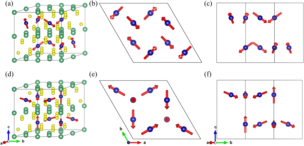
the assistance of SOC. As shown in Fig. 7(a), CoNb 3 S 6 has a hexagonal crystal structure
(nonmagnetic SG is No. 182, P6 3 22) with magnetic Co ion occupying 2d Wyckoff
positions. Interestingly, its all-in–all-out antiferromagnetic order forms a cubic structure in spin space, i.e., 𝐺 𝑠 = 4̅3𝑚. However, the corresponding MSG is P32’ with
only six symmetry elements because within the MSG framework, the spin rotation must
compromise the spatial rotation, implying that the cubic nature of spin symmetry is lost.
With 𝐺 0 = 𝑃6 3 22, the sublattice group 𝐿 0 = 𝑃2 1 (No. 4) forms a g-type normal subgroup with the subgroup indices 𝑖 𝑡 = 6 and 𝑖 𝑘 = 2 × 2 × 1 = 4, the latter of which corresponds to two-fold cell expansions along the x and y directions, i.e., {1|1 0 0} and
also belong to 𝐺 0 ⁄ 𝐿 0 . Overall, there are two possibilities of 24-element 𝐺 𝑠 being isomorphic to 𝐺 0 ⁄ 𝐿 0 i.e., 432 and ̅ 4 3𝑚, with each corresponding to one inequivalent mapping. Therefore, there are two nontrivial SSGs in total, labeled by (4.182.4.1) and
(4.182.4.2), respectively. In the case of CoNb 3 S 6 , real space {2 100 |0} operation couples spin space 𝑚 110 operation, rendering 𝐺 𝑠 = 4̅3𝑚 and thus a nontrivial SSG (4.182.4.2).
and {2 100 ‖1|0 1 0}. We note that the PG part of 𝐺 𝑇𝑆 forms a D 2 group in spin space. Therefore, the corresponding international notation is written as
the full SSG has 48 symmetry operations. Interestingly, such SSGs contain real space
and spin space symmetries from totally incompatible crystal systems, a scenario that is
impossible within the scope of MSG.
Fig. 7(b) shows the band structure of CoNb 3 S 6 calculated using DFT. Notably,
while PT is absent, the bands exhibit double degeneracy throughout the Brillouin zone.
Such a new form of spin degeneracy appears only in the framework of SSG, attributed 28 to the double-valued 2D co-irreps of the little co-group D 2 in spin space (the elements
in 𝐺 𝑇𝑆 leave k invariant) at any arbitrary k-points. Furthermore, the three perpendicular twofold spin rotation axes enforce any spin polarization components to be zero.
Therefore, the spin degeneracy/spin splitting induced by magnetic order in noncollinear
magnetic structures extends beyond the scope of MSGs, as only Tτ symmetry in the
spin translation group can be maintained when considering the MSGs. Consequently,
we summarize the complete criteria of spin splitting for noncollinear antiferromagnetic
orders, i.e., (i) the absence of PT, and (ii) the spin-space PG of the spin translation group
does not contain D n . This further highlights the importance of the enumeration and
representation theory of SSGs.
The noncoplanar magnetic order could lead to responses without the assistance of
SOC. For example, the anomalous Hall effect has long been attributed as a consequence
of SOC under time-reversal breaking [80]. On the other hand, the exchange field
induced by noncoplanar order could also induce anomalous Hall effect without SOC.
Instead of the topological Hall effect, we use the terminology of geometric Hall effect
to emphasize the sole origin of magnetic geometry. While the characteristic quantities
of noncoplanar magnets, e.g., scalar spin chirality [81] or band-resolved Berry
curvature [82], cannot fully describe the existence of the geometric Hall effect, we note
that due to the absence of SOC, the geometric Hall conductivity tensor can be fully
determined by SSG. For collinear and coplanar orders, the spin-only symmetry 𝑇𝑈 𝒏 (𝜋)
when integrating the Berry curvature over the Brillouin zone. Therefore, the anomalous
Hall effect in collinear or coplanar magnets (even for ferromagnets) must be a SOC
effect. However, for noncoplanar CoNb 3 S 6 , the PG symmetries of real-space part of the
SSG (62′2′) leave the z component of the magnetization invariant. Thus, an orbital
7(d), our DFT calculation obtains nonzero geometric Hall conductivity throughout the
Ω −1 cm −1 at the Fermi level, which is comparable to the largest anomalous Hall 29 conductivities in antiferromagnets with the assistance of SOC [83].
To conclude, we present a systematic study of the enumeration and the
representation theory of SSG applied to describe different magnetic configurations. By
using a group extension approach, our enumeration constructs a collection of over
100000 nontrivial SSGs, named by a four-index nomenclature. The International
notation system for SSGs is also developed. Furthermore, we derive the irreducible
projective co-representations of the little groups of the wavevectors within the SSG
framework, which is the foundation for understanding the symmetry-enforced
degeneracies in band spectra. To facilitate the search for SSG symmetries, we develop
an online program (https://findspingroup.com/) that can identify the SSG symmetries
of any given magnetic crystal. The SSG identification for all ~1970 experimentally
reported magnetic structures provided in the MAGNDATA database is also provided.
We then show representative material examples, including altermagnet RuO 2 ,
helimagnets CeAuAl 3 , and noncoplanar antiferromagnet CoNb 3 S 6 to illustrate their
SSG symmetries and the emergent properties beyond the MSG framework. Our work
further develops the group theory in describing materials with magnetic order, thereby
unlocking possibilities for future exploration into exotic phenomena within magnetic
materials.
Note added. During the finalization of our work, we became aware of related studies on the classification of spin space groups from Chen Fang’s and Zhi-Da Song’s groups
[84, 85]. In addition, we also noticed recent studies on symmetry analysis and search
of spin space groups [86, 87], as well as the representations of spin point groups [88].
Acknowledgements
We thank Chen Fang and Zhi-Da Song for helpful discussions. This work was supported by National Key R&D Program of China under Grant No. 2020YFA0308900, the 30
National Natural Science Foundation of China under Grant No. 12274194, Guangdong Provincial Key Laboratory for Computational Science and Material Design under Grant No. 2019B030301001, Shenzhen Science and Technology Program under Grant No. RCJC20221008092722009, the Science, Technology and Innovation Commission of Shenzhen Municipality (No. ZDSYS20190902092905285), Special Funds for the Cultivation of Guangdong College Students’ Scientific and Technological Innovation (No. pdjh2024c10202) and Center for Computational Science and Engineering of Southern University of Science and Technology.
31 Table I: Nontrivial SSGs for different crystal systems and different magnetic
configurations. “Collinear only” indicates nontrivial SSGs that only support collinear magnetic orders, i.e., 𝐺 𝑠 = 1 and ̅ 1 . Similarly, “Noncoplanar only” requires that 𝐺 𝑠 is
a polyhedral PG (T, T d , T h , O, and O h ). “Coplanar” contains nontrivial SSGs that support
coplanar magnetic orders.
Crystal system Collinear only Coplanar Noncoplanar only Total Triclinic (2) 5 55 0 60 Monoclinic (13) 78 3540 0 3618 Orthorhombic (59) 503 53734 0 54237 Tetragonal (68) 502 31185 0 31687 Trigonal (25) 83 2331 62 2476 Hexagonal (27) 137 7149 111 7397
Cubic (36) 113 840 184 1137 Total (230) 1421 98834 357 100612 32 Table II. The PG 𝐺 𝑠 in spin space for all the SSGs with the cell expansion limited to
𝑖 𝑘 ≤ 8. H-M symbol stands for Hermann-Mauguin symbol. H-M symbol Point group n 1, 2, 3, 4, 5, 6, 7, 8, 9, 10, 12, 14, 15, 16, 18, 20, 21, 24, 28, 30, 42 nm 3m, 5m, 7m, 9m, (15)m, (21)m nmm mm2, 4mm, 6mm, 8mm, (10)mm, (12)mm, (14)mm, (16)mm,
(18)mm, (20)mm, (24)mm, (28)mm, (30)mm, (42)mm -n -1, m, -3, -4, -5, -6, -7, -8, -9, -10, -12, -14. -15, -16, -18, -20. -21, -24,
-28, -30, -42, n/m 2/m, 4/m, 6/m, 8/m, (10)/m, (12)/m, (14)/m, (16)/m n2 32, 52, 72, 92, (15)2, (21)2 n22 222, 422, 622, 822, (10)22, (12)22, (14)22, (16)22, (18)22, (20)22,
(24)22, (28)22, (30)22, (42)22 -nm -3m, -5m, -7m, -9m, (-15)m, (-21)m, -n2m -42m, -62m, -82m, (-10)2m, (-12)2m, (-14)2m, (-16)2m, (-18)2m,
(-20)2m, (-24)2m, (-28)2m, (-30)2m, (-42)2m, n/mmm mmm, 4/mmm, 6/mmm, 8/mmm, (10)/mmm, (12)/mmm, (14)/mmm,
(16)/mmm, cubic 23, 432, m-3, -43m, m-3m 33 Table III. Symmetry operations and general positions of SSG (13.54.1.1) 𝑃 −1 𝑐 −1 𝑐 1 𝑎 .
In this table, a, b, and c represent the coordinates of a general position using the lattice
basis of the SSG; x, y, and z denote the corresponding components of the magnetic
moment using Cartesian coordinate.
Operation
Coordinates
a, b, c, x, y, z -a, -b, -c, x, y, z Operation
-a+1/2, -b, c,
x, y, z a+1/2, b, -c,
x, y, z 34 Coordinates a+1/2, -b, -c+1/2,
-x, -y, -z -a+1/2, b, c+1/2,
-x, -y, -z -a, b, -c+1/2,
-x, -y, -z a, -b, c+1/2, -x,
-y, -z
35
36
37
38
39
40
41
In Appendix, we begin in Sec. A by defining the SSGs, establishing connections
with the more familiar nonmagnetic SGs and MSGs. In Sec. B, we review the
International notation and Seitz notation for SGs and MSGs, and extend these notations
to describe SSGs. Next, in Sec. C, we introduce the nomenclature for t-type, k-type and
g-type SSGs and show how to obtain all group elements using International notation of
SSGs. These nonmenclatures are also integrated in our online platform
findspingroup.com. In Sec. D, the site symmetry groups and Wyckoff positions are
introduced into SSGs. The construction of a magnetic structure using site symmetry
groups are also explained. In Sec. E, we provide some details regarding the rep theory
of SSG, including the projective reps for SSGs, the decomposition of regular projective
reps using CSCO method and the modified Dimmock and Wheeler’s character sum rule.
In Sec. F, we derive the band reps of the little groups of k for collinear SSGs,
exemplified by RuO 2 . In Sec. G and H, we show the band reps of SSGs and the
comparison of those between SSGs and MSGs for coplanar CeAuAl 3 and noncoplanar
CoNb 3 S 6 , respectively. In Sec. I, we provide an example (RuO 2 ) of our online program
for SSG identification. Lastly, in Sec. J, we provide the computational methods for the
first-principles calculations.
42
| Abbreviation | Stands for |
|---|---|
| PG | point group |
| SG | space group |
| MPG | magnetic point group |
| MSG | magnetic space group |
| SPG | spin point group |
| SSG | spin space group |
| SOC | spin-orbit coupling |
| rep | representation |
| irrep | irreducible representation |
| co-rep | co-representation |
| co-irrep | irreducible co-representation |
| HM | Hermann-Mauguin Notation, International Notation |
| CSCO | complete set of commuting operators |
| DFT | density functional theory |
| 𝐺0 | SG, supergroup of 𝐿0 |
| 𝐿0 | normal subgroup of 𝐺0 |
| 𝑔𝑠 | operations in spin space |
| 𝑔𝑙 | operations in real space |
| 𝑅 | PG part of 𝑔𝑙 |
| 𝜏 | fractional translation part of 𝑔𝑙 |
| 𝕋 | translation group |
| 𝑃 | space inversion |
| 𝑇 | time reversal |
| 𝑈𝛼 (𝜃) | spin rotation of 𝜃-degree along the 𝛼 axis |
| 𝐶𝛽 (𝜃) | spatial rotation of 𝜃-degree along the 𝛽 axis |
| 𝑇(𝐺) | translation subgroup of SG 𝐺 |
| 𝑃(𝐺) | quotient group of 𝐺 with respect to the 𝑇(𝐺) |
𝐿 0 normal subgroup of 𝐺 0 𝑔 𝑠 operations in spin space 𝑔 𝑙 operations in real space
𝜏 fractional translation part of 𝑔 𝑙 𝕋 translation group
𝑃 space inversion
𝑇 time reversal
𝑇(𝐺) translation subgroup of SG 𝐺
𝑃(𝐺) quotient group of 𝐺 with respect to the 𝑇(𝐺)
43 𝑡 integral translation operation in translation group 𝕋 or 𝑇(𝐺)
|𝐺| order of group 𝐺
𝐺 𝑠 mapped PG in spin space
| 𝑡 | integral translation operation in translation group 𝕋 or 𝑇(𝐺) | ||||
|---|---|---|---|---|---|
| \ | 𝐺\ | order of group 𝐺 | |||
| 𝑖𝑡 | PG-index of \ | 𝑃(𝐺0 )\ | /\ | 𝑃(𝐿0 )\ | |
| 𝑖𝑘 | supercell index of \ | 𝑇(𝐺0 )\ | /\ | 𝑇(𝐿0 )\ | |
| 𝐺𝑠 | mapped PG in spin space | ||||
| 𝐺𝑆𝐺 | SG | ||||
| 𝐺𝑀𝑆 | MSG | ||||
| 𝐺𝑆𝑆 | SSG | ||||
| 𝐺𝑆𝑂 | spin-only group | ||||
| 𝐺𝑁𝑆 | nontrivial SSG | ||||
| 𝐿 | maximal unitary subgroup of 𝐺 | ||||
| 𝐺𝑘 | little group of 𝐺 at k point | ||||
| 𝐺̃𝑘 | the quotient group of 𝐺𝑘 with respect to translation group 𝕋 | ||||
| 𝐺̆𝑘 | little co-group of 𝐺 at k point | ||||
| 𝐺̆𝑘,∗ | central extension group of the 𝐺̆𝑘 | ||||
| 𝑍𝑔 | cyclic group of integers | ||||
| ̅̅̅̅ 𝐺̃ 𝑘 | intrinsic group of 𝐺̃𝑘 | ||||
| 𝑀𝑘 | projective irrep of the little group 𝐺𝑘 | ||||
| 𝑑𝑘 | irrep of 𝐺̃𝑘 | ||||
| 𝐷𝑘 | rep matrix of co-rep | ||||
| 𝐺𝑅 | SG of input structure without magnetic configurations | ||||
| 𝐺𝑆 | the quotient group of the PG of magnetic moment vectors | ||||
| with respect to the spin-only group | |||||
| {𝑔𝑠 (𝑎)𝑖 ‖𝑅𝑖 \ | 𝜏𝑖 (𝑎) } | SSG symmtry with i labels PG part 𝑅𝑖 in real space and (𝑎) | |||
| labels the corresponding translations and spin operations | |||||
| 𝜙(𝑔𝑠 (𝑎)𝑖 ) | rotation angle of 𝑔𝑠 (𝑎)𝑖 | ||||
| 𝑁𝐺 (𝐿) | normalizer of 𝐿 with respect to 𝐺 | ||||
| 𝑁𝐴+ (𝐿) | chirality-preserving affine normalizer of 𝐿 | ||||
| 𝐺 𝑇𝑆 | spin translation group | ||||
𝑀 𝑘 projective irrep of the little group 𝐺 𝑘
𝐷 𝑘 rep matrix of co-rep 𝐺 𝑅 SG of input structure without magnetic configurations 𝐺 𝑆 the quotient group of the PG of magnetic moment vectors
with respect to the spin-only group
𝑠 𝑖 ‖𝑅 𝑖 |𝜏 𝑖 } SSG symmtry with i labels PG part 𝑅 𝑖 in real space and (𝑎)
labels the corresponding translations and spin operations
𝑁 𝐺 (𝐿) normalizer of 𝐿 with respect to 𝐺 𝑁 𝐴 + (𝐿) chirality-preserving affine normalizer of 𝐿 𝐺 𝑇𝑆 spin translation group
44 𝐺 𝒒 site-symmetry group at 𝒒 point
𝑀 𝑇 transformation matrix 45
A. SGs, MSGs, SSGs and their representations ........................................................ 48
inequivalent mappings .......................................................................................... 49 3. Little group and little co-group ...................................................................... 52
Projective representation in ordinary SGs ..................................................... 53 6. Central extension ........................................................................................... 55 7. Co-representation ........................................................................................... 55 8. Dimmock and Wheeler’s character sum rule ................................................. 56 B. International notation and Seitz symbol ............................................................... 58
Viewing direction of SGs ............................................................................... 58 2. International symbols of SGs ......................................................................... 58 3. Seitz symbols in real space ............................................................................ 59 4. Seitz symbols in spin space............................................................................ 63 5. Representative symmetries for SGs ............................................................... 63 C. The nomenclature for t-type, k-type and g-type SSGs ......................................... 75
t-type SSG ...................................................................................................... 75
I. 65.136.1.1 ................................................................................................ 75 II. 47.221.1.2 ................................................................................................ 76 III. 13.54.1.1~13.54.1.6 ................................................................................. 78 2. k-type SSG ..................................................................................................... 80
I. 99.107.4.1 ................................................................................................ 81 II. 174.174.3.1 .............................................................................................. 82 3. g-type SSG ..................................................................................................... 84
I. 4.182.4.2 .................................................................................................. 85 II. 3.22.8.1 .................................................................................................... 87 D. Introduction to site-symmetry groups and Wyckoff positions of SSGs ................ 89
I. 13.54.1.1~13.54.1.6 ................................................................................. 90 2. k-type SSG ..................................................................................................... 95
I. 99.107.4.1 ................................................................................................ 95 3. g-type SSG ..................................................................................................... 97
I. 4.182.4.2 .................................................................................................. 97 E. Representation theory of SSG ............................................................................. 102
F. Band representations in collinear SSGs .............................................................. 112
Double-valued representation ...................................................................... 112 2. General rules for doubled degeneracy in SSGs ........................................... 113 3. Little (co)groups of altermagnet RuO 2 ........................................................ 115 4. Irreducible co-representations of RuO 2 ....................................................... 118 46 5. Comparison with the co-irreps of MSG ....................................................... 121 G. Band representations in coplanar SSGs .............................................................. 124
Irreducible co-representations of CeAuAl 3 at 𝑌(u,1/2,0) ............................ 125 2. Irreducible co-representations of CeAuAl3 ................................................. 131
H. Band representations in noncoplanar SSGs ........................................................ 139
I. Online program in SSG identification ................................................................ 149 J. First-principles methods...................................................................................... 152 47
We first discuss SGs, MSGs and SSGs in terms of their symmetry operations, as summarized in Table A1. SGs describe the geometry of a nonmagnetic material, or the Hamiltonian that does not contain the spin operator (nonmagnetic materials without SOC). Therefore, their symmetry operations include spatial symmorphic symmetry (pure spatial PG symmetry) {𝐶 n (𝜃), 𝐼𝐶 n (𝜃)|0} and spatial non-symmorphic symmetry
On the other hand, while MSGs and SSGs contains all the operations listed in Table A1, the specific manifestations of each row for the two types of groups are quite different. If no additional symmetry operations is introduced compared to ordinary SGs, the MSGs are often regarded as type I MSG (colorless group). If a MSG contains pure spin PG symmetry {𝑔 𝑠 ‖𝐸|0} where no spatial rotations or fractional translations 𝜏 are involved, 𝑔 𝑠 can only be time-reversal 𝑇, corresponding to a type-II MSG (grey group).
improper spin rotations 𝑈 n (𝜃) or 𝑇𝑈 n (𝜃) compatible with the spatial rotation 𝐶 n (𝜃) , corresponding to a type-III MSG (colored point group). If a MSG contains spin nonsymmorphic symmetry {𝑔 𝑠 ‖𝐸|𝜏} where a spin operation is combined with a fractional translation 𝜏, again, 𝑔 𝑠 can only be time-reversal 𝑇, corresponding to a type-IV MSG (colored lattice). In comparison, SSGs allow separated spatial and spin rotations, leading to much more symmetry operations that are not allowed by MSGs. Specifically,
configurations. In addition, spin non-symmorphic symmetry widely exists in spiral magnetic configurations with a k-type SSG. For example, the k-type SSG with 𝑖 𝑘 = 4
For general symmorphic symmetry and general non-symmorphic symmetry, MSG requires that 𝑔 𝑠 can only be proper or improper spin rotations 𝑈 n (𝜃) or 𝑇𝑈 n (𝜃) compatible with the spatial rotation 𝐶 n (𝜃) . In comparison, within the framework of SSG, 𝑔 𝑠 can be 𝑈 m (𝜙) or 𝑇𝑈 m (𝜙) with the rotational angle and axis not necessarily compatible with those of the spatial rotation.
48 Table A1: Six types of operations in SGs, MSGs and SSGs. For pure spin PG symmetry and spin non-symmorphic symmetry in MSGs, 𝑔 𝑠 can only be time-reversal 𝑇 ; for general symmorphic symmetry and general non-symmorphic symmetry in MSGs, 𝑔 𝑠 can only be proper or improper spin rotations 𝑈 n (𝜃) or 𝑇𝑈 n (𝜃) compatible with the spatial rotation 𝐶 n (𝜃).
Notation Spin PG Spatial PG
fractional translation √ √ √
inequivalent mappings
This part is devoted to explaining the mathematical procedure of finding inequivalent coset decompositions and inequivalent mappings between the quotient group 𝐺 0 ⁄ 𝐿 0 and the spin-space PG 𝐺 𝑠 , which is an essential step to eliminate equivalent SSGs in the enumeration process. Before getting into the details of the mathematical procedure, we first introduce some necessary concepts.
Chirality-preserving operations are symmetry operations that preserve the chirality of the object. Specifically, in three-dimensional (3D) Euclidean space ℝ 3 , the linear transformations form 3D orthogonal group 𝑂(3) = 𝑆𝑂(3) ∪ 𝑃𝑆𝑂(3), where 𝑃 represents space inversion. Elements of 𝑆𝑂(3) are regarded as chirality-preserving operations because their transformation matrices have a determinant of 1. Therefore, the chirality-preserving mappings ℝ 3 includes all translations, proper rotations, and screw rotations, yet excluding reflections, inversions, rotoinversions, and glide 49 reflections.
Affine transformation, or affine mapping, is a linear mapping method that perserves points, straight lines, and planes. After an affine transformation, although the Euclidean lengths and angles may change, sets of parallel lines remain parallel.
Normalizer. For a group 𝐺 and its subgroup 𝐿, the normalizer of 𝐿 with respect to 𝐺 denotes the set of elements 𝑔 ∈ 𝐺 that leave the subgroup of 𝐿 unchanged by conjugation:
Let us review establishment of SG briefly. In the enumeration of SG, The group 𝐺 0 and 𝐺 0′ belong to the same affine space-group type if an affine transformation 𝑎 ∈
holds. Here 𝑇(ℝ 3 ) contains all translations in ℝ 3 and 𝐺𝐿(3, 𝑅) denotes the 3D linear group whose entries of matrices are real numbers. However, there are only 219 affine space-group types in total as the rotation part of an affine transformation 𝑎 may have a negative determinant. In other words, it means that 𝑎 does not preserve the chirality of 𝐺 0 . Only when the affine transformation 𝑎 is required to be chirality-preserving during the mapping process, we can distinguish eleven pairs of enantiomorphic SGs (lefthanded versus right-handed structures), as shown in Table A2, and 230 = 219 + 11 crystallographic SG types are obtained [64].
To construct a SSG, the first step is to decompose a SG 𝐺 0 into its subgroups 𝐿 0 .
For two pairs (𝐺 0 , 𝐿 0 ) and (𝐺 0′ , 𝐿 ′ 0 ), it is obvious if 𝐺 0 and 𝐺 0′ belong to different SGs, as well as 𝐿 0 and 𝐿 ′ 0 , the coset decompositions and thus the resulting SSGs are different. On the other hand, even if both of (𝐺 0 , 𝐿 0 ) and (𝐺 0′ , 𝐿 ′ 0 ) cannot be distinguished just by their SGs, the coset decompositions of the two pairs may still be different. To provide a more detailed explanation, one can firstly transform 𝐿 0 and 𝐿 ′ 0 to the default setting of SGs so that they are identical (𝐿 0 = 𝐿 ′ 0 ). Then a chirality-preserving affine mapping 𝑎 in ℝ 3 is constructed to make the coset representatives of 𝐺 0 = 𝐿 0 ∪ 𝑔 1 𝐿 0 ∪. . .∪
Overall, the chirality-preserving affine normalizer 𝑁 𝐴 + (𝐿 0 ) was employed to find all inequivalent coset decompositions [64]. All affine mappings in ℝ 3 that map 𝐿 0 onto itself by conjugation and preserve its chirality form the chirality-preserving affine 50
Here, 𝑆𝐿(3, ℤ) denotes the 3D linear group whose entries of matrices are integers and determinant is of 1. Thus, two pairs (𝐺 0 , 𝐿 0 ) and ( 𝐺 0′ , 𝐿 0 ) are equivalent if their supergroups are conjugated under 𝑎 ∈ 𝑁 𝐴 + (𝐿 0 ):
The conclusion can be directly extended when considering the inclusion of spin
pairs are equivalent if they can be mapped onto each other by:
where 𝑁 𝐴 + (𝐺 0 ) is the chirality-preserving affine normalizer of 𝐺 0 and 𝑁 𝑂(3) (𝐺 𝑠 ) is the normalizer of 𝐺 𝑠 in orthogonal group 𝑂(3).
The abovementioned mathematical procedure of identifying all inequivalent coset decompositions and inequivalent mappings for constructing SSGs using Eq. (A4) to (A6) is performed by Magma, which is a large, well-supported software package designed for computations in abstract mathematical objects. It basically provides nearly all the significant algorithms for finite groups and finitely presented infinite groups.
Table A2: Eleven pairs of enantiomorphic SGs
51
The translation generators of a SG 𝐺 determine its Bravais lattice and also its Brillouin zone (BZ). Points in the BZ are denoted by 𝑘 in momentum space. The action of 𝑔 = {𝑅|𝜏} ∈ 𝐺 on 𝑘 is 𝑔𝑘 = 𝑅𝑘 , where translation 𝜏 leaves 𝑘 invariant. All elements in a SG 𝐺 that keeps a reciprocal vector 𝑘 invariant form a group named the little group of 𝑘. Since we focus on the properties of Bloch states under band theory, where Bloch states are labeled by reciprocal vectors 𝑘, the little group of 𝑘 is of great importance. The PG part of a little group is called a little co-group. Such concept is introduced because the theory of projective rep maps the derivation of irreps of a little group to the derivation of projective irreps of the corresponding little co-group, in which lattice translation is neglected and the fractional translation is included in factor systems (the details will be discussed later).
A representation of group 𝐺 is formally defined as a homomorphism from 𝐺 to the group form by general linear transformations on a vector space 𝑉, i.e., the general linear group 𝐺𝐿(𝑉) . The matrix forms of those linear transformations are called representation matrices. In quantum physics, group rep is considered with a certain group of quantum states as a basis. Under this situation, a group rep can be simply understood as the matrix form of all symmetry operators. This method allows us to describe the symmetry of quantum systems with easily manipulated linear algebra. Generally, by basis transformation, a vector space can be separated into subspaces such that all vectors of one subspace are only transformed into each other. This allows us to block diagonalize the full rep matrices of all group elements simultaneously and view the full rep as the direct sum of reps on every subspace. Those reps which have rep matrices that cannot be block diagonalized by any basis transformation are called irreducible representations. In quantum physics, irreps describe the degeneracy of quantum states and encode basic symmetry information of quantum states, e.g., parity, 52 angular momentum numbers, etc.
A regular representation is defined as the rep by using the group space as the rep space, where the group elements function as both the operators and as the bases for the space. It is a particularly interesting set of matrices that forms a reducible rep of the group 𝐺, which can be block-diagonalized to give all irreps of the group. The matrices of the regular rep are constructed with the following relation:
The multiplicity 𝑎 𝑗 of each irrep in the regular rep can be calculated to be equal to its dimension 𝑙 𝑗 :
Namely,
where 𝜒 𝑗 (𝑅), 𝐷 𝑗 (𝑅) represent the character and the rep matrix for the irrep 𝑗 of the group 𝐺, respectively, while 𝜒 𝑟𝑒𝑔 (𝑅), 𝐷 𝑟𝑒𝑔 (𝑅) represent the character and the rep matrix for the reducible rep of the regular rep, repsectively. 𝐸, 𝑔, 𝑋 stand for the identity, the order of the group 𝐺 and the similarity transformation, respectively.
In summary, the regular rep contains each irrep a number of times equal to the dimensionality of the rep, i.e., the n-dimensional irreps appears n times in regular reps.
In SGs, the fractional translations usually bring complexities to the reps, leading to extra degeneracies, etc. The reps of any little groups of 𝑘 can be obtained by the projective reps of the corresponding little co-group. To elaborate on this, we first consider a little group 𝐺 𝑘 with the coset form with respect to translation group 𝕋 to be:
The rep of 𝕋 with a basis of Bloch functions at momentum 𝑘 is already known with the form 𝑒𝑥𝑝 (−𝑖𝑘 ⋅ 𝜏). Thus, to get a full list of irreps of 𝐺 𝑘 , all we need to do is to derive
One can naively think the rep of the coset representatives as the rep of the corresponding little co-group 𝐺̆ 𝑘 = (𝑅 1 , 𝑅 2 , … , 𝑅 𝑛 ) . However, they are not always the same because 53 of the possible nonsymmorphic translation 𝜏 𝑖 , i.e., if we assume 𝑅 𝑖 𝑅 𝑗 = 𝑅 𝑘 , the product
where 𝜏 𝑖𝑗 = 𝜏 𝑖 + 𝑅 𝑖 𝜏 𝑗 − 𝜏 𝑘 . Therefore, the nonsymmorphic translation 𝜏 𝑖 and 𝜏 𝑗 could result in a lattice translation {𝐸|𝜏 𝑖𝑗 } beyond the {𝑅 𝑘 |𝜏 𝑘 }. Thus, the product relation of a rep 𝑑 𝑘 at 𝑘 point should obey the following:
which exhibit an additional phase factor 𝑒𝑥𝑝 (−𝑖𝑘 ⋅ 𝜏 𝑖𝑗 ).
Strictly speaking, the group of rep matrices could be much larger than the group of coset representatives 𝐺̃ 𝑘 , or the little co-group 𝐺̆ 𝑘 . These rep matrices should include
rep matrices could cover little co-group 𝐺̆ 𝑘 multiple times because one 𝑅 𝑘 could combine with different translations. To simplify the problem, we can use the theory of projective rep to “mod” the influence of nonsymmorphic translations and get all irreps of 𝐺 𝑘 by deriving the corresponding irreducible projective reps.
Projective representation is formally defined as follows: For a group 𝐻 consisting of elements ℎ 𝑖 , where 𝑖 ranges from 1 to |𝐻|, a non-singular matrix function Δ on group 𝐻 is a projective representation of 𝐻 if it satisfies the following rule:
For each group product ℎ 𝑖 ℎ 𝑗 = ℎ 𝑘 , there exists a scalar function 𝜇(ℎ 𝑖 , ℎ 𝑗 ) on the group elements ℎ 𝑖 , ℎ 𝑗 , obeying that
The function 𝜇(ℎ 𝑖 , ℎ 𝑗 ) is called a factor system for the projective rep Δ.
In the problem of multiple reps of {𝑅 𝑖 𝑅 𝑗 |𝜏 𝑖 + 𝑅 𝑖 𝜏 𝑗 } discussed above, we can see that the product of rep 𝑑 𝑘 does not follow the rule of Eq. (A13) because 𝜏 𝑖𝑗 = 𝜏 𝑖 + 𝑅 𝑖 𝜏 𝑗 − 𝜏 𝑘 is dependent on 𝜏 𝑘 . To solve this, we define the projective rep corresponding
Under this definition, one can show that
𝑒𝑥𝑝(−𝑖𝐾 𝑖 ⋅ 𝜏 𝑗 ) form a projective irrep of the little group 𝐺 𝑘 . The set 𝑀 𝑘 forms an irrep 54
completely dependent on {𝑅 𝑖 |𝜏 𝑖 } and {𝑅 𝑗 |𝜏 𝑗 }. Consequently, to get all irreps 𝑑 𝑘 of 𝐺̃ 𝑘 , one needs to derive all the corresponding projective irreps 𝑀 𝑘 of 𝐺̆ 𝑘 . In practice, 𝑀 𝑘 is obtained by central extension method, which is introduced in the following.
We now encounter two possibilities regarding the multiplier factor system. One case is all the factor system 𝜇(𝑅 𝑖 , 𝑅 𝑗 ) = 1, and hence the irreps of little group 𝐺 𝑘 and the little co-group 𝐺̆ 𝑘 coincide. If one of following three conditions is reached, the factor system maps into unity: (1) 𝐺 is a symmorphic SG; (2) 𝐺 𝑘 is a symmorphic group; (3) k lies inside the first Brillouin zone.
Another case is that the factor system 𝜇(𝑅 𝑖 , 𝑅 𝑗 ) can take multiple values, when 𝐺 𝑘 is a non-symmorphic group and k lies on the Brillouin zone boundary. In such situation, a typical treatment, named central extension, to obtain the projective reps is to find the reps of a new abstract group 𝐺̆ 𝑘,∗ = 𝐺̆ 𝑘 × 𝑍 𝑔 , where 𝑍 𝑔 denotes the cyclic group of
table of the operations in 𝐺̆ 𝑘∗ is determined by the following relationship:
where (𝑅 𝑖 , 𝛼) are group elements of the central extension of little cogroup 𝐺̆ 𝑘,∗ and 𝛼 ∈
Following this approach, 𝐺̆ 𝑘,∗ can be identified with one isomorphic abstract group and the irreps can be determined. Of all irreps, we only focus on the right irreps
can construct the character table of the projective irreps of 𝐺 𝑘 . More details and specific examples can be found in Ref. [2].
In magnetic materials, group description usually involves antiunitary operations that include time-reversal operator T. These operations contain a complex conjugation operation that transforms any complex number into its complex conjugate. A famous 55
example of band degeneracy induced by antiunitary groups is the so-called Kramers degeneracy. However, a comprehensive understanding of the transformation of quantum states under antiunitary groups requires more than just knowledge of Kramers degeneracy. To achive this, we must first know the unitary rep matrices under antiunitary groups. Owing to the properties of antiunitary operations, the matrix representatatives 𝐷 do not obey the ordinary multiplication relations associated with unitary groups, but rather satisfy the following equations:
where 𝑢, 𝑢 1 , 𝑢 2 represent any unitary operation, while 𝑎, 𝑎 1 , 𝑎 2 represent any antiunitary operation of the same magnetic group, 𝐷 ∗ is the complex conjugate rep of
𝐷. This kind of rep is named as “co-representation” by Wigner. The theory of co-rep is
useful for analyzing extra degeneracies caused by antiunitary operations and the
corresponding degenerate states.
Following the above, the co-irreps of MSGs are constructed. For any little group
we only need to classify the induced co-irreps from the irreps of the maximal unitary
subgroup 𝐿̃ 𝑘 𝑀𝑆 using the Dimmock and Wheeler’s sum rule as summarized in three cases:
dimension, in this case, no extra degeneracy is introduced.
dimension, in this case, the degeneracy is doubled.
56
can be stick together under the antiunitary operators.
We summarize the Dimmock and Wheeler’s sum rule as
where 𝜒 is the character of 𝑑.
57 (A19)
In International notation, SGs are designated by a symbol 𝐵𝑔 1 𝑔 2 𝑔 3 that combines the SG symmetry with a uppercase letter describing the centering of the Bravais lattice.
Specifically, 𝐵 is denoted by P for primitive lattice, A, B, C for base-centered lattice, I
for body-centered lattice, F for face-centered lattice and R for rhombohedral lattice.
The subsequent three symbols 𝑔 1 𝑔 2 𝑔 3 represent the representative symmetry operations when projected along one of the high symmetry directions of the crystal.
The high symmetry directions of different crystal systems are shown as follows:
| order | Triclinic | Monoclinic | Orthorhombic | Tetragonal | Trigonal | Hexagonal | Cubic | |||
|---|---|---|---|---|---|---|---|---|---|---|
| 1 | [010] | [100] | [100] | [001] | [001] | [001] | [001] | [100] | ||
| 2 | [010] | [010] | [100] | [100] | [100] | [100] | [111] | |||
| 3 | [001] | [001] | [110] | [110] | [210] | [210] | [110] | |||
| For example, the four letters of 𝑃32 12 (153) represents a primitive lattice, consisting of a 3-fold rotation along the [001] direction with a 2/3c translation, identity along the [100] direction and a 2-fold rotation along the [210] direction. 2. International symbols of SGs Here we list International symbols and their corresponding symmetry operations used for SGs, such as rotation, mirror, rotation-inversion in the PG, as well as glide, screw in the SG. Table B2: Symbols of SG using International notation, including rotation axes, mirror planes, screw axes and glide planes. | For example, the four letters of 𝑃32 12 (153) represents a primitive lattice, consisting of a 3-fold rotation along the [001] direction with a 2/3c translation, identity along the [100] direction and a 2-fold rotation along the [210] direction. 2. International symbols of SGs Here we list International symbols and their corresponding symmetry operations used for SGs, such as rotation, mirror, rotation-inversion in the PG, as well as glide, screw in the SG. Table B2: Symbols of SG using International notation, including rotation axes, mirror planes, screw axes and glide planes. | For example, the four letters of 𝑃32 12 (153) represents a primitive lattice, consisting of a 3-fold rotation along the [001] direction with a 2/3c translation, identity along the [100] direction and a 2-fold rotation along the [210] direction. 2. International symbols of SGs Here we list International symbols and their corresponding symmetry operations used for SGs, such as rotation, mirror, rotation-inversion in the PG, as well as glide, screw in the SG. Table B2: Symbols of SG using International notation, including rotation axes, mirror planes, screw axes and glide planes. | For example, the four letters of 𝑃32 12 (153) represents a primitive lattice, consisting of a 3-fold rotation along the [001] direction with a 2/3c translation, identity along the [100] direction and a 2-fold rotation along the [210] direction. 2. International symbols of SGs Here we list International symbols and their corresponding symmetry operations used for SGs, such as rotation, mirror, rotation-inversion in the PG, as well as glide, screw in the SG. Table B2: Symbols of SG using International notation, including rotation axes, mirror planes, screw axes and glide planes. | For example, the four letters of 𝑃32 12 (153) represents a primitive lattice, consisting of a 3-fold rotation along the [001] direction with a 2/3c translation, identity along the [100] direction and a 2-fold rotation along the [210] direction. 2. International symbols of SGs Here we list International symbols and their corresponding symmetry operations used for SGs, such as rotation, mirror, rotation-inversion in the PG, as well as glide, screw in the SG. Table B2: Symbols of SG using International notation, including rotation axes, mirror planes, screw axes and glide planes. | For example, the four letters of 𝑃32 12 (153) represents a primitive lattice, consisting of a 3-fold rotation along the [001] direction with a 2/3c translation, identity along the [100] direction and a 2-fold rotation along the [210] direction. 2. International symbols of SGs Here we list International symbols and their corresponding symmetry operations used for SGs, such as rotation, mirror, rotation-inversion in the PG, as well as glide, screw in the SG. Table B2: Symbols of SG using International notation, including rotation axes, mirror planes, screw axes and glide planes. | For example, the four letters of 𝑃32 12 (153) represents a primitive lattice, consisting of a 3-fold rotation along the [001] direction with a 2/3c translation, identity along the [100] direction and a 2-fold rotation along the [210] direction. 2. International symbols of SGs Here we list International symbols and their corresponding symmetry operations used for SGs, such as rotation, mirror, rotation-inversion in the PG, as well as glide, screw in the SG. Table B2: Symbols of SG using International notation, including rotation axes, mirror planes, screw axes and glide planes. | For example, the four letters of 𝑃32 12 (153) represents a primitive lattice, consisting of a 3-fold rotation along the [001] direction with a 2/3c translation, identity along the [100] direction and a 2-fold rotation along the [210] direction. 2. International symbols of SGs Here we list International symbols and their corresponding symmetry operations used for SGs, such as rotation, mirror, rotation-inversion in the PG, as well as glide, screw in the SG. Table B2: Symbols of SG using International notation, including rotation axes, mirror planes, screw axes and glide planes. | For example, the four letters of 𝑃32 12 (153) represents a primitive lattice, consisting of a 3-fold rotation along the [001] direction with a 2/3c translation, identity along the [100] direction and a 2-fold rotation along the [210] direction. 2. International symbols of SGs Here we list International symbols and their corresponding symmetry operations used for SGs, such as rotation, mirror, rotation-inversion in the PG, as well as glide, screw in the SG. Table B2: Symbols of SG using International notation, including rotation axes, mirror planes, screw axes and glide planes. | For example, the four letters of 𝑃32 12 (153) represents a primitive lattice, consisting of a 3-fold rotation along the [001] direction with a 2/3c translation, identity along the [100] direction and a 2-fold rotation along the [210] direction. 2. International symbols of SGs Here we list International symbols and their corresponding symmetry operations used for SGs, such as rotation, mirror, rotation-inversion in the PG, as well as glide, screw in the SG. Table B2: Symbols of SG using International notation, including rotation axes, mirror planes, screw axes and glide planes. | For example, the four letters of 𝑃32 12 (153) represents a primitive lattice, consisting of a 3-fold rotation along the [001] direction with a 2/3c translation, identity along the [100] direction and a 2-fold rotation along the [210] direction. 2. International symbols of SGs Here we list International symbols and their corresponding symmetry operations used for SGs, such as rotation, mirror, rotation-inversion in the PG, as well as glide, screw in the SG. Table B2: Symbols of SG using International notation, including rotation axes, mirror planes, screw axes and glide planes. |
| Name | Name | Name | Name | Notation | Notation | Remark | Remark | Remark | Remark | Remark |
| identity | identity | identity | identity | 1 | 1 | |||||
planes, screw axes and glide planes. Name Notation identity 1 58 Remark inversion -1 rotation n n-fold rotation rotation-inversion -n n-fold rotation followed by an inversion mirror m reflection in a plane mirror plane ⊥ to n-fold axes n/m screw 𝑛 𝑖 n-fold rotation followed by i/n fraction
glide mirror (combination of a mirror and a fraction translation) axial glide a tranlation of a/2
b tranlation of b/2 c tranlation of c/2 diagnonal glide n tranlation of (a+b)/2, (b+c)/2, (a+c)/2 diamond glide d tranlation of (a+b)/4, (b+c)/4, (a+c)/4
with perpendicular direction. For instance, the SG Aem2 (39) has a mirror parallel to a
with a translation of b/2 and a centering fraction translation of (b+c)/2, resulting in the
mirror parallel to a with a translation of c/2. As a consequence, Aem2 can be referred
as Abm2 and Acm2 simultaneously. Therefore, the symbol “e” is employed for such
planes. Similar situations can be found in Aea2 (41), Cmce (64), Cmme (67) and Ccce
(68).
International notations only provide description of representative group elements
for denoting SGs. In order to denote all group elements, Seitz symbols are introduced.
We generalized the Seitz symbol {𝑅|𝜏} in SGs to {𝑔 𝑠 ‖𝑅|𝜏} in SSGs, where 𝑔 𝑠 , 𝑅, and 𝜏 represent spin rotation, space rotation and translation, respectively. However, due to
the complexity of translational supercell, the PG in spin space will not always have the
same crystal systems as the space part. For example, the space part of 4.182.4.2
(CoNb 3 S 6 ) belongs to the hexagonal system (𝑃6 3 22), while the spin part belongs to the cubic system (-43m). Therefore, we define the space part of SSG symmetry in the lattice 59 basis, i.e., a, b, c, while the spin part of SSG symmetry is defined in Cartesian
coordinate system, i.e., x, y, z. The nomenclature for the symbol 𝑅 in real space is
shown below:
The symbol 𝑅 signifies the operations of identity and space inversion with 1 and -
1, respectively. The symbol m represents mirror operations, while the symbols n (n = 2,
3, 4, 6) are utilized for n-fold rotations, and -n (n = 3, 4, 6) denote rotation-inversion
operations. For rotations and rotation-inversions of order higher than 2, a superscript i
is used to indicate the number of applications of rotations and the subscript hkl is used
to denote the characteristic direction of the operation. For example, the 4 3 001 represents an anticlockwise rotation of 270-degree along the [001] crystallographic direction.
The following two tables list all Seitz symbols for the SG operations in the seven
crystal systems. Here 𝑎⃗ , 𝑏⃗⃗ and 𝑐⃗ denote the lattice basis vectors, while a, b and c
represent the coordination using the lattice basis a, b, c.
Table B3: Seitz symbols for PG part of space-group symmetry operations of the cubic,
tetragonal, orthorhombic, monoclinic and triclinic crystal systems.
No. Seitz symbol Axes Coordination
a,b,c 60
25 -1
-a,-b,-c 61
Table B4: Seitz symbols for PG part of space-group symmetry operations of the
hexagonal and trigonal crystal systems.
No. Seitz symbol Axes Coordination
13 -1
a,b,c -a,-b,-c 62
We extend the nomenclature for the symbol 𝑔 s in spin space: The symbol 𝑔 s is 1 and -1 for identity and time reversal, respectively. The symbols n (n = 2, 3, 4, 5, 6, 7, 8 …) are used for n-fold spin rotations. The improper spin rotation
represents the time reversal followed by proper spin rotations, including m for the
combination of the time reversal and 2-fold rotation and -n for the combination of the
time reversal and n-fold rotation. Similarly, a superscript i is used to indicate the number
of applications of rotations and the subscript hkl denote the characteristic direction of
the operation. For example, 5 2 001 stands for 144-degree rotation along the [001] direction. We include three axial directions [100], [010], [001], six face-diagonal
directions [110], [1-10], [101], [10-1], [011], [01-1] and four body-diagonal direction
[111], [-11-1], [1-1-1], [-1-11]. In addition, the subscript 𝜃 ∈ (0, 𝜋) is employed to label
the specific direction in the x-y plane. For example, the 2 𝜃 label the in-plane 2-fold rotation around the in-plane 𝜃-direction axis with respect to x direction (shown in Fig.
B1).
63 Now we present the complete list of SG 𝐵𝑔 1 𝑔 2 𝑔 3 with International notation and their corresponding Seitz symbols, which are used to label SSGs according to their
crystal systems.
First we list the detailed centering-type fractional translation 𝑏 1 , 𝑏 2 , 𝑏 3 for SG in various Bravais lattices, i.e., the corresponding symmetry operations of 𝐵.
Table B5: The centering-type fractional translation 𝑏 1 , 𝑏 2 , 𝑏 3 for SG in different Bravais lattices, which is used as default sequence in g-type SSG.
Secondly, we show the following three representative symbols, 𝑔 1 𝑔 2 𝑔 3 , within 230 SGs 𝐵𝑔 1 𝑔 2 𝑔 3 , categorized into triclinic, monoclinic, orthorhombic, tetragonal, trigonal, hexagonal and cubic crystal systems.
Table B6: Table of symbol-group element correspondence in SGs of triclinic crystal
systems, with no viewing direction is used.
Table B7: Table of symbol-group element correspondence in SGs of monoclinic crystal
systems, with viewing direction of [010] in International notation.
64 𝑔 3
10 P2/m 11 P2 1 /m 12 C2/m 13 P2/c 14 P2 1 /c 15 C2/c
Table B8: Table of symbol-group element correspondence in SGs of orthorhombic
crystal systems, with viewing direction of [100], [010] and [001] in International
notation.
65
66
Table B9: Table of symbol-group element correspondence in SGs of tetragonal crystal
systems, with viewing direction of [001], [100] and [110] in International notation.
67 𝑔 3 83 84 85 86 P4/m P4 2 /m P4/n P4 2 /n
68
128 P4/mnc 129 P4/nmm 130 P4/ncc 131 P4 2 /mmc
69
132 P4 2 /mcm 133 134 135
Table B10: Table of symbol-group element correspondence in SGs of trigonal crystal
systems, with viewing direction of [001], [100] and [210] in International notation.
70 𝑔 3
Table B11: Table of symbol-group element correspondence in SGs of hexagonal crystal
systems, with viewing direction of [001], [100] and [210] in International notation.
71 𝑔 3
Table B12: Table of symbol-group element correspondence in SGs of hexagonal crystal
systems, with viewing direction of [100], [111] and [110] in International notation.
72 g 3
73
74
Below we give the guidance for constructing nontrivial SSG 𝐺 𝑁𝑆 using the nomenclature of t-type, k-type and g-type SSG.
I. 65.136.1.1
Following Table B9, 𝑃 −1 4 2 / 1 𝑚 −1 𝑛 1 𝑚 (65.136.1.1) can be generated using
elements are listed below. Here a, b, c and x, y, z coordination correspond to space
coordination and vector of magnetic moment, respectively, 𝜏 = (1/2 1/2 1/2).
Table C1: General positions of 𝑃 −1 4 2 / 1 𝑚 −1 𝑛 1 𝑚 (65.136.1.1).
Seitz
Coordination Seitz
a, b, c,
x, y, z -a, -b, c,
x, y, z b, a, -c,
x, y, z -b, -a, -c,
x, y, z -a, -b, -c,
x, y, z a, b, -c,
x, y, z -b, -a, c,
x, y, z
| {41 001 ‖43 001 \ | 1/2 1/2 1/4} | b+1/2, -a+1/2, c+1/4, -y, x, z |
|---|---|---|
| {41 001 ‖𝑚010 \ | 1/2 1/2 1/4} | a+1/2, -b+1/2, c+1/2, -y, x, z |
| {41 001 ‖𝑚100 \ | 1/2 1/2 1/4} | -a+1/2, b+1/2, c+1/4, -y, x, z |
| {41 001 ‖𝑚110 \ | 1/2 1/2 1/4} | -b+1/2, -a+1/2, c+1/4, -y, x, z |
| {41 001 ‖𝑚1−10 \ | 1/2 1/2 1/4} | b+1/2, a+1/2, c+1/4, -y, x, z |
| {2001 ‖1\ | 0 0 1/2} | a, b, c+1/2, -x, -y, z |
| {2001 ‖2001 \ | 0 0 1/2} | -a, -b, c+1/2, -x, -y, z |
| {2001 ‖41 001 \ | 0 0 1/2} | -b, a, c+1/2, -x, -y, z |
| {2001 ‖43 001 \ | 0 0 1/2} | b, -a, c+1/2, -x, -y, z |
| {2001 ‖𝑚010 \ | 0 0 1/2} | a, -b, c+1/2, -x, -y, z |
| {2001 ‖𝑚100 \ | 0 0 1/2} | -a, b, c+1/2, -x, -y, z |
| {2001 ‖𝑚110 \ | 0 0 1/2} | -b, -a, c+1/2, -x, -y, z |
| {2001 ‖𝑚1−10 \ | 0 0 1/2} | b, a, c+1/2, -x, -y, z |
| {43 001 ‖1\ | 1/2 1/2 1/4} | a+1/2, b+1/2, c+3/4, y, -x, z |
| {43 001 ‖2001 \ | 1/2 1/2 1/4} | -a+1/2, -b+1/2, c+3/4, y, -x, z |
| {43 001 ‖41 001 \ | 1/2 1/2 1/4} | -b+1/2, a+1/2, c+3/4, y, -x, z |
| {43 001 ‖43 001 \ | 1/2 1/2 1/4} | b+1/2, -a+1/2, c+3/4, y, -x, z |
| {43 001 ‖𝑚010 \ | 1/2 1/2 1/4} | a+1/2, -b+1/2, c+3/4, y, -x, z |
| {43 001 ‖𝑚100 \ | 1/2 1/2 1/4} | -a+1/2, b+1/2, c+3/4, y, -x, z |
| {43 001 ‖𝑚110 \ | 1/2 1/2 1/4} | -b+1/2, -a+1/2, c+3/4, y, -x, z |
| {43 001 ‖𝑚1−10 \ | 1/2 1/2 1/4} | b+1/2, a+1/2, c+3/4, y, -x, z |
x, y, z -x, -y, -z As shown in Table C1, we can conclude that SSG with 𝐺 𝑠 = −1 only supports
collinear magnetic structures, supposing that no inequivalent magnetic ion in the
magnetic cell. Take the collinear antiferromagnet RuO 2 as an example, whose nontrivial
which is named as ∞𝑚 1 in International notation. As a result, for collinear
II. 47.221.1.2
3 1 𝑚 Now we turn to a more complex one, 𝑃 1 𝑚 001 −3 010 𝑚 (47.221.1.2). {𝑚
100 |0},
{−3 1 111 |0}, {𝑚 110 |0} are obtained following Table B12. Now we perform the coset
According to representative symmetry operations of 47.221.1.2, {1‖𝑚 100 |0} ,
Then we make the direct product of {𝐸‖𝐿 0 } and {𝑔 𝑆 ‖𝑔 𝛼 }, all the general positions are then obtained and listed in Table C2.
3 1 𝑚 Table C2: General positions of 𝑃 1 𝑚 001 −3 010 𝑚 (47.221.1.2).
Seitz Coordination
76
77
III. 13.54.1.1~13.54.1.6
All general positions of 13.54.1.1 to 13.54.1.6 are also listed below in Table C3 to
C8. The International notations for 13.54.1.1 to 13.54.1.6 are 𝑃 −1 𝑐 −1 𝑐 1 𝑎 ,
respectively.
Table C3: General positions of 𝑃 −1 𝑐 −1 𝑐 1 𝑎 (13.54.1.1).
Seitz
Coordination
a, b, c, x, y, z -a, -b, -c, x, y, z Seitz
78 Coordination a+1/2, -b, -c+1/2,
-x, -y, -z -a+1/2, b, c+1/2,
-x, -y, -z
-a+1/2, -b, c,
x, y, z a+1/2, b, -c,
x, y, z -a, b, -c+1/2,
-x, -y, -z a, -b, c+1/2, -x,
-y, -z Table C4: General positions of 𝑃 2 001 𝑐 2 001 𝑐 1 𝑎 (13.54.1.2).
Seitz
Coordination
a, b, c, x, y, z -a, -b, -c, x, y, z Seitz
-a+1/2, -b, c,
x, y, z a+1/2, b, -c,
x, y, z Coordination a+1/2, -b, -c+1/2,
-x, -y, z -a+1/2, b, c+1/2,
-x, -y, z -a, b, -c+1/2,
-x, -y, z a, -b, c+1/2,
-x, -y, z Table C5: General positions of 𝑃 𝑚 001 𝑐 𝑚 001 𝑐 1 𝑎 (13.54.1.3).
Seitz
Coordination
a, b, c, x, y, z -a, -b, -c, x, y, z Seitz
-a+1/2, -b, c,
x, y, z a+1/2, b, -c,
x, y, z
Coordination a+1/2, -b, -c+1/2,
x, y, -z -a+1/2, b, c+1/2,
x, y, -z -a, b, -c+1/2,
x, y, -z a, -b, c+1/2,
x, y, -z Table C6: General positions of 𝑃 −1 𝑐 1 𝑐 −1 𝑎 (13.54.1.4).
Seitz
Coordination
a, b, c, x, y, z -a, -b, -c, Seitz
79 Coordination a+1/2, -b, -c+1/2,
-x, -y, -z -a+1/2, b, c+1/2, x, y, z
-x, -y, -z -a, b, -c+1/2,
x, y, z a, -b, c+1/2,
x, y, z -a+1/2, -b, c,
-x, -y, -z a+1/2, b, -c, -x, -y, -z Table C7: General positions of 𝑃 2 001 𝑐 1 𝑐 2 001 𝑎 (13.54.1.5).
Seitz
Coordination
a, b, c, x, y, z -a, -b, -c, x, y, z Seitz
-a, b, -c+1/2,
x, y, z a, -b, c+1/2,
x, y, z Coordination a+1/2, -b, -c+1/2,
-x, -y, z -a+1/2, b, c+1/2,
-x, -y, z -a+1/2, -b, c,
-x, -y, z a+1/2, b, -c,
-x, -y, z Table C8: General positions of 𝑃 𝑚 001 𝑐 1 𝑐 𝑚 001 𝑎 (13.54.1.6).
Seitz
Coordination
a, b, c, x, y, z -a, -b, -c, x, y, z Seitz
-a, b, -c+1/2,
x, y, z a, -b, c+1/2,
x, y, z
Coordination a+1/2, -b, -c+1/2,
x, y, -z -a+1/2, b, c+1/2,
x, y, -z -a+1/2, -b, c,
x, y, -z a+1/2, b, -c,
x, y, -z 2. k-type SSG In the BNS setting, MSGs are constructed from space group 𝐿 0 . This can be achieved by adding a "primed sublattice" generated by an operation that combines time-
inversion with a fractional translation to describe the “reversal” of spin between 80
different nonmagnetic unit cells. The type-IV group is constructed by 𝑀 𝐼𝑉 = 𝐿 0 + 𝑇𝜏𝐿 0 , where 𝜏 is the mentioned translation. The k-type SSG can be seen as the multi-color
externsion of MSG. In this case, due to the decoupling of spin space and lattice space,
a point group in spin space is used to describe the propagation vector in the enlarged
for k-type SSG under 𝐿 0 basis. In this vein, the k-type SSG is directly constructed from the direct product of sublattice SG {𝐸‖𝐵𝑔 1 𝑔 2 𝑔 3 } and additional spin translation group
I. 99.107.4.1
Seitz Coordination
81
II. 174.174.3.1
Now we show why we use the 𝐿 0 basis, rather than the 𝐺 0 basis for k-type SSG. The 𝐿 0 basis depict the magnetic primitive cell, while the 𝐺 0 basis sometimes give a 3 1 larger primitive cell. Now we take 𝑃 1 −6 001 (2/3 1/3 0) (174.174.3.1) as an example.
82 Under 𝐿 0 basis, the sublattice SG is 𝐿 0 = 𝑃 − 6 , the spin translation group is
listed in Table C10.
Seitz Coordination
𝐿 0 basis to 𝐺 0 basis. Then three spin translation operation is transformed into {1‖1|0},
83
3 1 Fig. C1: Magnetic primitive cell of 𝑃 1 −6 001 (2/3 1/3 0) (174.174.3.1) under 𝐿
0
basis (black line) and under 𝐺 0 basis (orange line).
It is clear that the magnetic cell under 𝐺 0 basis is three times larger than 𝐿 0 basis as shown in Fig. C1. In other words, the magnetic cell under 𝐿 0 basis is also the minimum periodic unit cell, while the magnetic cell under 𝐺 0 basis is sometimes larger than the previous, depending on the transform matrix.
combined with centering-type fractional translation 𝑏 1 , 𝑏 2 , 𝑏 3 . The spin translation
{𝑔 𝑠 7 ‖𝑏 3 }. The sequence of 𝑏 1 , 𝑏 2 , 𝑏 3 for different Bravais lattices is given in Table B5.
84 When 𝐵 = 𝑃 for primitive lattice, 𝑔 𝑠 7 , 𝑔 𝑠 8 , 𝑔 𝑠 9 are omitted. Below we show several
examples of g-type SSG.
I. 4.182.4.2
the spin translation group 𝐺 𝑇𝑆 =
Seitz Coordination
85
86 II. 3.22.8.1
In 𝐺 0 basis, the Bravais-centering fractional translation 𝑏 1 𝑏 2 𝑏 3 can also combine with nontrivial spin operation. Below we show how to construct the full SSG from the
The spin translation group 𝐺 𝑇𝑆 for 3.22.8.1 can be constructed from {2 001 ‖1|0 0 1},
The integral translations along three basis vector of 𝐺 0 for 3.22.8.1 are
(3.22.8.1).
Seitz Coordination
87
88
This section aims to define the site-symmetry group 𝐺 𝒒 at a point q in a crystal
that is invariant under a SSG 𝐺, which comprises spin-space symmetry operations 𝑔 𝑖 :
where 𝑔 𝑠 𝑖 represents a spin-space unitary/antiunitary symmetry operation
encompassing the identity, a rotation, time reversal, or time reversal followed by
rotation; 𝑅 𝑖 denotes a real-space symmetry operation that is either the identity, inversion, a rotation or a rotation-inversion; and 𝜏 𝑖 is a real-space pure translation.
Given a point q in a crystal, the action of 𝑔 𝑖 on q can be expressed as:
where only 𝑅 𝑖 and 𝜏 𝑖 act on q due to the invariance of spatial coordinates under both
𝑞 time revesal and spin-space rotation. Those operations 𝑔
𝑖 that leave the point invariant
form the site-symmetry group 𝐺 𝒒 , i.e., 𝑔 𝑖𝑞 𝒒 = 𝒒. Additionally, the elements 𝑔 𝛼 ∈ 𝐺 but
𝑔 𝛼 ∉ 𝐺 𝒒 in magnetic primitive cell form the cosets 𝐺/𝐺 𝒒 , which is the set of points
positions, and n represents the multiplicity. Therefore, the site-symmetry group 𝐺 𝒒 is a
finite subgroup of the SSG 𝐺 , i.e., 𝐺 𝒒 ⊂ 𝐺 . It is important to note that 𝐺 𝒒 does not
contain any element in the form of {𝑔 𝑠 𝑖 ‖1|𝜏 𝑖 } or {1‖1|𝜏 𝑖 }, where 1 is the identity and
In the following discussion, we explore the relationship between nontrivial site-
SSG and nontrivial SPG. For t-type SSG, 𝐺 𝒒 is found to be isomorphic to one of the
598 nontivial SPGs detailed in Litvin’s work [18]. Specially, for k-type and g-type SSGs,
stablize any point in position space. Thus, 𝐺 𝒒 can not contain any operation in the form
of {𝑔 𝑠 𝑖 ‖1|𝜏 𝑖 } . In summary, for t-type, k-type and g-type SSG, 𝐺 𝒒 always exhibits
isomorphism to one of the 598 nontivial SPGs. In contrast, the spin translation group 89 𝐺 𝑇𝑆 always present in the coset 𝐺/𝐺 𝒒 , which tells the difference of volumn between magnetic unit cell and nonmangnetic unit cell.
Next we show how to obtain Wyckoff positions in t-type, k-type and g-type SSG.
using Eq. (3). Since the site 𝒒 is invariant under any spin-space operation 𝑔 𝑠 𝑖 , and the
magnetic cell of t-type SSG is the same with nonmagnetic cell. Then Eq. (3) can be
viewed as
when act on the site 𝒒. In other word, the t-type SSG shares the same Wyckoff-position
multiplicities and coordinates with SG 𝐺 0 . Besides, the site-symmetry group 𝐺 𝒒 is also
I. 13.54.1.1~13.54.1.6
Here we use 13.54.1.1~13.54.1.6 as an example, telling about the construction of
Wyckoff positions, site-symmetry groups and construct realistic magnetic structures
using these SSGs.
As stated before, the t-type SSG shares the same Wyckoff-position multiplicities
and coordinates with SG 𝐺 0 . Below is these information about 𝐺 0 = 𝑃𝑐𝑐𝑎 (No. 54).
Table D1: Wyckoff positions for SG 𝐺 0 = 𝑃𝑐𝑐𝑎 (No. 54) from WYCKPOS at Bilbao Crystallography Server [89].
| WP | Site-SG | Coordinates |
|---|---|---|
| 4a | -1 | (0, 0, 0), (1/2, 0, 0), (0, 0, 1/2), (1/2, 0, 1/2) |
| 4b | -1 | (0, 1/2, 0), (1/2, 1/2, 0), (0, 1/2, 1/2), (1/2, 1/2, 1/2) |
| 4c | 2 | (0, b, 1/4), (1/2, -b, 1/4), (0, -b, 3/4), (1/2, b, 3/4) |
90
| Seitz | Coordination | |
|---|---|---|
| {1‖1\ | 0} | a, b, c, x, y, z |
| {2001 ‖1\ | 0 0 1} | a, b, c+1, -x, -y, z |
| {41 001 ‖1\ | 1/2 0 1/2} | a+1/2, b, c+1/2, -y, x, z |
| {43 001 ‖1\ | 1/2 0 3/2} | a+1/2, b, c+3/2, y, -x, z |
| {−1‖1\ | 1/2 1/2 1} | a+1/2, b+1/2, c+1, -x, -y, -z |
| {𝑚001 ‖1\ | 1/2 1/2 0} | a+1/2, b+1/2, c, x, y, -z |
| {−41 001 ‖1\ | 0 1/2 3/2} | a, b+1/2, c+3/2, y, -x, -z |
| {−43 001 ‖1\ | 0 1/2 1/2} | a, b+1/2, c+1/2, -y, x, -z |
| {1‖2001 \ | 0} | -a, -b, c, x, y, z |
| {2001 ‖2001 \ | 0 0 1} | -a, -b, c+1, -x, -y, z |
| {41 001 ‖2001 \ | 1/2 0 1/2} | -a+1/2, -b, c+1/2, -y, x, z |
| {43 001 ‖2001 \ | 1/2 0 3/2} | -a+1/2, -b, c+3/2, y, -x, z |
| {−1‖2001 \ | 1/2 1/2 1} | -a+1/2, -b+1/2, c+1, -x, -y, -z |
| {𝑚001 ‖2001 \ | 1/2 1/2 0} | -a+1/2, -b+1/2, c, x, y, -z |
| {−41 001 ‖2001 \ | 0 1/2 3/2} | -a, -b+1/2, c+3/2, y, -x, -z |
For the t-type SSG, only the site-symmetry group and the magnetic moment on
each coordinate should be added for constructing Wyckoff-positions of SSG. Here we
choose some representative sites to show the construction of site-SSG of 𝑃 −1 𝑐 −1 𝑐 1 𝑎
(13.54.1.1).
Table D2: Representative sites for all Wyckoff positions for 𝐺 0 = 𝑃𝑐𝑐𝑎 (No. 54).
WP Representative Site-symmetry group
Here we show all symmetry operations of 13.54.1.1
Following above, we map the spin operation with space part to obtain Wyckoff
positions of 𝑃 −1 𝑐 −1 𝑐 1 𝑎 (13.54.1.1), and we calculate the constrain on magnetic
moments.
Table D3: Representative sites for all Wyckoff positions for 𝑃 −1 𝑐 −1 𝑐 1 𝑎 (13.54.1.1).
13.54.1.1
4a Representative Site-symmetry group
91 notation 1 −1 magnetic moments (x, y, z)
Following these procedure, the Wyckoff positions of 𝑃 −1 𝑐 −1 𝑐 1 𝑎 (13.54.1.1) are
constructed and shown in Table D4. Similarly, Wyckoff positions of
13.54.1.2~13.54.1.6 are also constructed and shown in Table D5 to D9.
Table D4: Wyckoff positions for 𝑃 −1 𝑐 −1 𝑐 1 𝑎 (13.54.1.1).
WP Site-SSG
| Operation | Coordinates | Operation | Coordinates | ||
|---|---|---|---|---|---|
| {1‖1\ | 0} | x, a, b, y, z c, | {−1‖2100 \ | 1/2 0 1/2} | a+1/2, -b, -c+1/2, -x, -y, -z |
| {1‖ − 1\ | 0} | -a, x, -b, y, z -c, | {−1‖𝑚100 \ | 1/2 0 1/2} | -a+1/2, b, c+1/2, -x, -y, -z |
| {1‖2001 \ | 1/2 0 0} | -a+1/2, x, y, -b, z c, | {−1‖2010 \ | 0 0 1/2} | -a, -x, b, -y, -c+1/2, -z |
| {1‖𝑚001 \ | 1/2 0 0} | a+1/2, x, y, b, z -c, | {−1‖𝑚010 \ | 0 0 1/2} | a, -b, -y, c+1/2, -z -x, |
(-a, b, -c+1/2 | -x, -y, -z), (a+1/2, -b, -c+1/2 | -x, -y, -z),
(-a, -b, -c | x, y, z), (a+1/2, b, -c | x, y, z), (a, -b, c+1/2 | -x, -y, -z), (-a+1/2, b, c+1/2 | -x, -y, -z)
Table D5: Wyckoff positions for 𝑃 2 001 𝑐 2 001 𝑐 1 𝑎 (13.54.1.2).
WP Site-SSG
Coordinates (0, 0, 0 | x, y, z), (1/2, 0, 0 | x, y, z), (0, 0, 1/2 | -x, -y, z), (1/2, 0, 1/2 | -x, -y, z) (0, 1/2, 0 | x, y, z), (1/2, 1/2, 0 | x, y, z), 92 (0, 1/2, 1/2 | -x, -y, z), (1/2, 1/2, 1/2 | -x, -y, z)
(0, b, 1/4 | 0, 0, z), (1/2, -b, 1/4 | 0, 0, z), (0, -b, 3/4 | 0, 0, z), (1/2, b, 3/4 | 0, 0, z)
(a, b, c | x, y, z), (-a+1/2, -b, c | x, y, z), 8f
(a, -b, c+1/2 | -x, -y, z), (-a+1/2, b, c+1/2 | -x, -y, z)
Table D6: Wyckoff positions for 𝑃 𝑚 001 𝑐 𝑚 001 𝑐 1 𝑎 (13.54.1.3).
WP Site-SSG
| Seitz | Coordination | Seitz | Coordination | ||
|---|---|---|---|---|---|
| {1‖1\ | 0} | x, a, b, y, z c, | {−1‖41 001 \ | 𝜏} | -b+1/2, a+1/2, c+1/2, -x, -y, -z |
| {1‖2001 \ | 0} | -a, x, -b, y, z c, | {−1‖43 001 \ | 𝜏} | b+1/2, -a+1/2, c+1/2, -x, -y, -z |
| {1‖2110 \ | 0} | b, x, a, y, -c, z | {−1‖2100 \ | 𝜏} | a+1/2, -b+1/2, -c+1/2, -x, -y, -z |
| {1‖21−10 \ | 0} | -b, x, -a, y, z -c, | {−1‖2010 \ | 𝜏} | -a+1/2, b+1/2, -c+1/2, -x, -y, -z |
| {1‖ − 1\ | 0} | -a, x, -b, y, z -c, | {−1‖−41 001 \ | 𝜏} | b+1/2, -a+1/2, -c+1/2, -x, -y, -z |
| {1‖𝑚001 \ | 0} | a, x, b, y, -c, z | {−1‖−43 001 \ | 𝜏} | -b+1/2, a+1/2, -c+1/2, -x, -y, -z |
| {1‖𝑚110 \ | 0} | -b, x, y, -a, z c, | {−1‖𝑚100 \ | 𝜏} | -a+1/2, b+1/2, c+1/2, -x, -y, -z |
| {1‖𝑚1−10 \ | 0} | b, a, c, | {−1‖𝑚010 \ | 𝜏} | a+1/2, -b+1/2, c+1/2, |
| (0, 1/2, 1/2 \ | -x, -y, z), (1/2, 1/2, 1/2 \ | -x, -y, z) | ||||||||
|---|---|---|---|---|---|---|---|---|---|---|
| 4c | 2001 2 | (0, (0, -b, b, 1/4 3/4 \ | \ | 0, 0, 0, 0, z), z), (1/2, (1/2, -b, b, 3/4 1/4 \ | \ | 0, 0, 0, 0, z) z), | ||||
| 4d | 1 2 | (3/4, (1/4, 0, 0, -c c \ | \ | x, x, y, y, z), z), (3/4, (1/4, 0, 0, -c+1/2 c+1/2 \ | \ | -x, -x, -y, -y, z) z), | ||||
| 4e | 1 2 | (1/4, 1/2, c \ | x, y, z), (3/4, 1/2, -c+1/2 \ | -x, -y, z), (3/4, 1/2, -c \ | x, y, z), (1/4, 1/2, c+1/2 \ | -x, -y, z) | ||||
| 8f | 1 1 | (-a, (a, -b, b, (-a, -c+1/2 (a, c+1/2 -b, b, c \ | -c \ | -x, \ | -x, x, \ | x, -y, -y, y, y, z), z), z), z), (-a+1/2, (-a+1/2, (a+1/2, (a+1/2, -b, -b, b, b, c+1/2 -c -c+1/2 c \ | \ | x, x, y, y, \ | \ | -x, z), z), -x, -y, -y, z) z), |
| Table D6: Wyckoff positions for 𝑃𝑚001 𝑐𝑚001 𝑐1 𝑎 (13.54.1.3). | Table D6: Wyckoff positions for 𝑃𝑚001 𝑐𝑚001 𝑐1 𝑎 (13.54.1.3). | Table D6: Wyckoff positions for 𝑃𝑚001 𝑐𝑚001 𝑐1 𝑎 (13.54.1.3). | ||||||||
| WP | Site-SSG | Coordinates | ||||||||
| 4a | 1 −1 | (0, (0, 0, 1/2 0, 0 \ | \ | x, x, y, y, -z), z), (1/2, (1/2, 0, 0, 1/2 0 \ | x, \ | x, y, y, z), -z) | ||||
| 4b | 1 −1 | (0, 1/2, 0 \ | x, y, z), (1/2, 1/2, 0 \ | x, y, z), (0, 1/2, 1/2 \ | x, y, -z), (1/2, 1/2, 1/2 \ | x, y, -z) | ||||
| 4c | 𝑚001 2 | (0, (0, -b, b, 1/4 3/4 \ | \ | x, x, y, y, 0), 0), (1/2, (1/2, -b, b, 3/4 1/4 \ | \ | x, x, y, y, 0) 0), | ||||
| 4d | 1 2 | (1/4, 0, c \ | x, y, z), (3/4, 0, -c+1/2 \ | x, y, -z), (3/4, 0, -c \ | x, y, z), (1/4, 0, c+1/2 \ | x, y, -z) | ||||
| 4e | 1 2 | (1/4, 1/2, c \ | x, y, z), (3/4, 1/2, -c+1/2 \ | x, y, -z), (3/4, 1/2, -c \ | x, y, z), (1/4, 1/2, c+1/2 \ | x, y, -z) | ||||
| 8f | 1 1 | (a, b, c \ | x, y, z), (-a+1/2, -b, c \ | x, y, z), (-a, b, -c+1/2 \ | x, y, -z), (a+1/2, -b, -c+1/2 \ | x, y, -z), (-a, -b, -c \ | x, y, z), (a+1/2, b, -c \ | x, y, z), (a, -b, c+1/2 \ | x, y, -z), (-a+1/2, b, c+1/2 \ | x, y, -z) |
| Table D7: Wyckoff positions for 𝑃−1 𝑐1 𝑐−1 𝑎 (13.54.1.4). | Table D7: Wyckoff positions for 𝑃−1 𝑐1 𝑐−1 𝑎 (13.54.1.4). | Table D7: Wyckoff positions for 𝑃−1 𝑐1 𝑐−1 𝑎 (13.54.1.4). | ||||||||
| WP | Site-SSG | Coordinates | ||||||||
| 4a | 1 −1 | (0, 0, 0 \ | x, y, z), (1/2, 0, 0 \ | -x, -y, -z), | ||||||
| x, y, z | -x, -y, -z | ||||
|---|---|---|---|---|---|
| {1‖2010 \ | 0 0 1/2} | -a, x, b, y, -c+1/2, z | {−1‖2001 \ | 1/2 0 0} | -a+1/2, -x, -y, -b, -z c, |
| {1‖𝑚010 \ | 0 0 1/2} | a, -b, x, y, c+1/2, z | {−1‖𝑚001 \ | 1/2 0 0} | a+1/2, -x, -y, b, -z -c, |
| Table C7: General positions of 𝑃2001 𝑐1 𝑐2001 𝑎 (13.54.1.5). | |||||
| Seitz | Coordination | Seitz | Coordination | ||
| {1‖1\ | 0} | x, a, b, y, z c, | {2001 ‖2100 \ | 1/2 0 1/2} | a+1/2, -b, -c+1/2, -x, -y, z |
| {1‖ − 1\ | 0} | -a, x, -b, y, z -c, | {2001 ‖𝑚100 \ | 1/2 0 1/2} | -a+1/2, b, c+1/2, -x, -y, z |
| {1‖2010 \ | 0 0 1/2} | -a, x, b, y, -c+1/2, z | {2001 ‖2001 \ | 1/2 0 0} | -a+1/2, -x, -y, -b, z c, |
| {1‖𝑚010 \ | 0 0 1/2} | a, -b, x, y, c+1/2, z | {2001 ‖𝑚001 \ | 1/2 0 0} | a+1/2, -x, -y, b, z -c, |
| Table C8: General positions of 𝑃𝑚001 𝑐1 𝑐𝑚001 𝑎 (13.54.1.6). | Table C8: General positions of 𝑃𝑚001 𝑐1 𝑐𝑚001 𝑎 (13.54.1.6). | Table C8: General positions of 𝑃𝑚001 𝑐1 𝑐𝑚001 𝑎 (13.54.1.6). | Table C8: General positions of 𝑃𝑚001 𝑐1 𝑐𝑚001 𝑎 (13.54.1.6). | ||
| Seitz | Coordination | Seitz | Coordination | ||
| {1‖1\ | 0} | x, a, b, y, z c, | {𝑚001 ‖2100 \ | 1/2 0 1/2} | a+1/2, -b, -c+1/2, x, y, -z |
| {1‖ − 1\ | 0} | -a, x, -b, y, z -c, | {𝑚001 ‖𝑚100 \ | 1/2 0 1/2} | -a+1/2, b, c+1/2, x, y, -z |
| {1‖2010 \ | 0 0 1/2} | -a, x, b, y, -c+1/2, z | {𝑚001 ‖2001 \ | 1/2 0 0} | -a+1/2, x, y, -z -b, c, |
| {1‖𝑚010 \ | 0 0 1/2} | a, -b, x, y, c+1/2, z | {𝑚001 ‖𝑚001 \ | 1/2 0 0} | a+1/2, x, y, b, -z -c, |
(-a, b, -c+1/2 | x, y, z), (a+1/2, -b, -c+1/2 | -x, -y, -z),
(-a, -b, -c | x, y, z), (a+1/2, b, -c | -x, -y, -z), (a, -b, c+1/2 | x, y, z), (-a+1/2, b, c+1/2 | -x, -y, -z)
Table D8: Wyckoff positions for 𝑃 2 001 𝑐 1 𝑐 2 001 𝑎 (13.54.1.5).
WP Site-SSG
| {1‖2010 \ | 0} | -a, b, -c, x, y, z |
|---|---|---|
| {1‖2001 \ | 0} | -a, -b, c, x, y, z |
| {1‖ − 1\ | 0} | -a, -b, -c, x, y, z |
| {1‖𝑚100 \ | 0} | -a, b, c, x, y, z |
| {1‖𝑚010 \ | 0} | a, -b, -c, x, y, z |
| {1‖𝑚001 \ | 0} | a, b, -c, x, y, z |
| {31 001 ‖31 111 \ | 0} | c, a, b, -(x+√3y)/2, (√3x-y)/2, z |
| {31 001 ‖31 1−11 \ | 0} | c, -a, -b, -(x+√3y)/2, (√3x-y)/2, z |
| {31 001 ‖31 1−1−1 \ | 0} | -c, -a, b, -(x+√3y)/2, (√3x-y)/2, z |
| {31 001 ‖31 11−1 \ | 0} | -c, a, -b, -(x+√3y)/2, (√3x-y)/2, z |
| {31 001 ‖−31 111 \ | 0} | -c, -a, -b, -(x+√3y)/2, (√3x-y)/2, z |
| {31 001 ‖−31 1−11 \ | 0} | -c, a, b, -(x+√3y)/2, (√3x-y)/2, z |
| {31 001 ‖−31 1−1−1 \ | 0} | c, a, -b, -(x+√3y)/2, (√3x-y)/2, z |
| {31 001 ‖−31 11−1 \ | 0} | c, -a, b, -(x+√3y)/2, (√3x-y)/2, z |
| {32 001 ‖3111 2 \ | 0} | b, c, a, (-x+√3y)/2, -(√3x+y)/2, z |
| {32 001 ‖31−11 2 \ | 0} | -b, -c, a, (-x+√3y)/2, -(√3x+y)/2, z |
| {32 001 ‖31−1−1 2 \ | 0} | -b, c, -a, (-x+√3y)/2, -(√3x+y)/2, z |
| {32 001 ‖311−1 2 \ | 0} | b, -c, -a, (-x+√3y)/2, -(√3x+y)/2, z |
| {32 001 ‖−3111 2 \ | 0} | -b, -c, -a, (-x+√3y)/2, -(√3x+y)/2, z |
| {32 001 ‖−31−11 2 \ | 0} | b, c, -a, (-x+√3y)/2, -(√3x+y)/2, z |
| {32 001 ‖−31−1−1 2 \ | 0} | b, -c, a, (-x+√3y)/2, -(√3x+y)/2, z |
| {32 001 ‖ − 311−1 2 \ | 0} | -b, c, a, (-x+√3y)/2, -(√3x+y)/2, z |
| {𝑚010 ‖2110 \ | 0} | b, a, -c, x, -y, z |
| {𝑚010 ‖21−10 \ | 0} | -b, -a, -c, x, -y, z |
| {𝑚010 ‖41 001 \ | 0} | -b, a, c, x, -y, z |
| {𝑚010 ‖43 001 \ | 0} | b, -a, c, x, -y, z |
| {𝑚010 ‖𝑚110 \ | 0} | -b, -a, c, x, -y, z |
| {𝑚010 ‖𝑚1−10 \ | 0} | b, a, c, x, -y, z |
| {𝑚010 ‖−41 001 \ | 0} | b, -a, -c, x, -y, z |
| {𝑚010 ‖−43 001 \ | 0} | -b, a, -c, x, -y, z |
(-a, b, -c+1/2 | x, y, z), (a+1/2, -b, -c+1/2 | -x, -y, z),
(-a, -b, -c | x, y, z), (a+1/2, b, -c | -x, -y, z), (a, -b, c+1/2 | x, y, z), (-a+1/2, b, c+1/2 | -x, -y, z)
Table D9: Wyckoff positions for 𝑃 𝑚 001 𝑐 1 𝑐 𝑚 001 𝑎 (13.54.1.6).
94 WP Site-SSG
Coordinates (0, 0, 0 | x, y, z), (1/2, 0, 0 | x, y, -z), (0, 0, 1/2 | x, y, z), (1/2, 0, 1/2 | x, y, -z) (0, 1/2, 0 | x, y, z), (1/2, 1/2, 0 | x, y, -z), (0, 1/2, 1/2 | x, y, z), (1/2, 1/2, 1/2 | x, y, -z)
(a, b, c | x, y, z), (-a+1/2, -b, c | x, y, -z),
(-a, b, -c+1/2 | x, y, z), (a+1/2, -b, -c+1/2 | x, y, -z),
(-a, -b, -c | x, y, z), (a+1/2, b, -c | x, y, -z), (a, -b, c+1/2 | x, y, z), (-a+1/2, b, c+1/2 | x, y, -z)
dependencies on the Wyckoff positions in the SG 𝐺 0 , which is similar to the Type-IV MSGs in the BNS setting. This complication arise from the spin translation operations
unit cell of a crystal compared to the nonmagnetic unit cell of SG 𝐺 0 . To construct the Wyckoff positions of k-type SSGs, the Wyckoff positions of SG 𝐺 0 , the transformation
position in k-type SSG will be an integer multiple of the index 𝑖 𝑘 when compared to the nonmagnetic primitive cell of SG 𝐺 0 . Here the transformation matrix 𝑀 T is introduced in order to suit the 𝐿 0 basis of k-type SSGs.
I. 99.107.4.1 95
First, we list the Wyckoff positions of SG 𝐺 0 = 𝐼4mm (No. 107) in Table D10.
Table D10: Wyckoff positions for SG 𝐺 0 = 𝐼4mm (No. 107) from WYCKPOS at Bilbao Crystallography Server [89].
| WP | Site-SSG | Coordinates | ||||||||
|---|---|---|---|---|---|---|---|---|---|---|
| 4a | 1 −1 | (0, (0, 0, 0, 1/2 0 \ | \ | x, x, y, y, z), z), (1/2, (1/2, 0, 0, 1/2 0 \ | x, \ | x, y, y, -z), -z) | ||||
| 4b | 1 −1 | (0, 1/2, 0 \ | x, y, z), (1/2, 1/2, 0 \ | x, y, -z), (0, 1/2, 1/2 \ | x, y, z), (1/2, 1/2, 1/2 \ | x, y, -z) | ||||
| 4c | 1 2 | (0, (0, -b, b, 1/4 3/4 \ | \ | x, x, y, y, z), z), (1/2, (1/2, -b, b, 3/4 1/4 \ | \ | x, x, y, y, -z) -z), | ||||
| 4d | 𝑚001 2 | (3/4, (1/4, 0, 0, -c c \ | \ | x, x, y, y, 0), 0), (3/4, (1/4, 0, 0, -c+1/2 c+1/2 \ | \ | x, x, y, y, 0) 0), | ||||
| 4e | 𝑚001 2 | (1/4, 1/2, c \ | x, y, 0), (3/4, 1/2, -c+1/2 \ | x, y, 0), (3/4, 1/2, -c \ | x, y, 0), (1/4, 1/2, c+1/2 \ | x, y, 0) | ||||
| 8f | 1 1 | (a, b, c \ | x, y, z), (-a+1/2, -b, c \ | x, y, -z), (-a, b, -c+1/2 \ | x, y, z), (a+1/2, -b, -c+1/2 \ | x, y, -z), (-a, -b, -c \ | x, y, z), (a+1/2, b, -c \ | x, y, -z), (a, -b, c+1/2 \ | x, y, z), (-a+1/2, b, c+1/2 \ | x, y, -z) |
1 Next, Wyckoff positions and site-SSGs for 𝑃 1 4 1 𝑚 1 𝑚 4
(99.107.4.1) are constructed using the transformation matrix
(99.107.4.1) are shown in Table D11.
Coordinates WP Site-SSG (0, 0, 0 | x, y, z) + (1/2, 1/2, 1/4 | -y, x, z)
96
| 16d | 1 𝑚 | (a, 0, c), (-a, 0, c), (0, a, c), (0, -a, c) | ||||||||||||||||||
|---|---|---|---|---|---|---|---|---|---|---|---|---|---|---|---|---|---|---|---|---|
| 32e | 1 1 | (a, (a, -b, b, c), c), (-a, (-a, -b, b, c), c), (-b, (-b, -a, a, c), c), (b, (b, -a, a, c) c) | ||||||||||||||||||
| 3. g-type SSG Similar to the k-type SSGs, the Wyckoff positions in g-type SSGs have more complicated dependencies on the Wyckoff positions in the SG 𝐺0 , which is similar to the Type-IV MSGs in the OG setting. Since now we must use the 𝐺0 basis to maintain the most spatial rotation part. This complication arise from the spin translation operations {𝑔𝑠𝑖 ‖1\ | 𝜏𝑖 } in g-type SSG 𝐵𝑔𝑠1 𝑔1 𝑔𝑠2 𝑔2 𝑔𝑠3 𝑔3 \ | (𝑔𝑠4 , 𝑔𝑠5 , 𝑔𝑠6 ; 𝑔𝑠7 , 𝑔𝑠8 , 𝑔𝑠9 ) , which enlarges the magnetic unit cell of a crystal compared to the nonmagnetic unit cell of SG 𝐺0 . To construct the Wyckoff positions of k-type SSGs, the Wyckoff positions of SG 𝐺0 and the spin translation group 𝐺 𝑇𝑆 = {{1‖1\ | 0}, {𝑔𝑠1 ‖1\ | 𝜏1 }, … , {𝑔𝑠𝑛−1 ‖1\ | 𝜏𝑛−1 }} are employed. Here the transformation matrix 𝑀T is no more necessary since the g-type SSGs are under 𝐺0 basis. I. 4.182.4.2 Wyckoff positions of the g-type SSG 𝑃32 −11−1 63 𝑚110 2𝑚011 2 \ | (2001 , 2100 , 1)(4.182.4.2) are constructed from Wyckoff positions of SG 𝐺0 = 𝑃63 22 (No. 182) shown in Table D12. Table D12: Wyckoff positions for SG 𝐺0 = 𝑃63 22 (No. 182) from WYCKPOS at Bilbao Crystallography Server [89]. | 3. g-type SSG Similar to the k-type SSGs, the Wyckoff positions in g-type SSGs have more complicated dependencies on the Wyckoff positions in the SG 𝐺0 , which is similar to the Type-IV MSGs in the OG setting. Since now we must use the 𝐺0 basis to maintain the most spatial rotation part. This complication arise from the spin translation operations {𝑔𝑠𝑖 ‖1\ | 𝜏𝑖 } in g-type SSG 𝐵𝑔𝑠1 𝑔1 𝑔𝑠2 𝑔2 𝑔𝑠3 𝑔3 \ | (𝑔𝑠4 , 𝑔𝑠5 , 𝑔𝑠6 ; 𝑔𝑠7 , 𝑔𝑠8 , 𝑔𝑠9 ) , which enlarges the magnetic unit cell of a crystal compared to the nonmagnetic unit cell of SG 𝐺0 . To construct the Wyckoff positions of k-type SSGs, the Wyckoff positions of SG 𝐺0 and the spin translation group 𝐺 𝑇𝑆 = {{1‖1\ | 0}, {𝑔𝑠1 ‖1\ | 𝜏1 }, … , {𝑔𝑠𝑛−1 ‖1\ | 𝜏𝑛−1 }} are employed. Here the transformation matrix 𝑀T is no more necessary since the g-type SSGs are under 𝐺0 basis. I. 4.182.4.2 Wyckoff positions of the g-type SSG 𝑃32 −11−1 63 𝑚110 2𝑚011 2 \ | (2001 , 2100 , 1)(4.182.4.2) are constructed from Wyckoff positions of SG 𝐺0 = 𝑃63 22 (No. 182) shown in Table D12. Table D12: Wyckoff positions for SG 𝐺0 = 𝑃63 22 (No. 182) from WYCKPOS at Bilbao Crystallography Server [89]. | 3. g-type SSG Similar to the k-type SSGs, the Wyckoff positions in g-type SSGs have more complicated dependencies on the Wyckoff positions in the SG 𝐺0 , which is similar to the Type-IV MSGs in the OG setting. Since now we must use the 𝐺0 basis to maintain the most spatial rotation part. This complication arise from the spin translation operations {𝑔𝑠𝑖 ‖1\ | 𝜏𝑖 } in g-type SSG 𝐵𝑔𝑠1 𝑔1 𝑔𝑠2 𝑔2 𝑔𝑠3 𝑔3 \ | (𝑔𝑠4 , 𝑔𝑠5 , 𝑔𝑠6 ; 𝑔𝑠7 , 𝑔𝑠8 , 𝑔𝑠9 ) , which enlarges the magnetic unit cell of a crystal compared to the nonmagnetic unit cell of SG 𝐺0 . To construct the Wyckoff positions of k-type SSGs, the Wyckoff positions of SG 𝐺0 and the spin translation group 𝐺 𝑇𝑆 = {{1‖1\ | 0}, {𝑔𝑠1 ‖1\ | 𝜏1 }, … , {𝑔𝑠𝑛−1 ‖1\ | 𝜏𝑛−1 }} are employed. Here the transformation matrix 𝑀T is no more necessary since the g-type SSGs are under 𝐺0 basis. I. 4.182.4.2 Wyckoff positions of the g-type SSG 𝑃32 −11−1 63 𝑚110 2𝑚011 2 \ | (2001 , 2100 , 1)(4.182.4.2) are constructed from Wyckoff positions of SG 𝐺0 = 𝑃63 22 (No. 182) shown in Table D12. Table D12: Wyckoff positions for SG 𝐺0 = 𝑃63 22 (No. 182) from WYCKPOS at Bilbao Crystallography Server [89]. |
| WP | Site-SG | Coordinates | ||||||||||||||||||
| 2a | 321 | (0, 0, 0), (0, 0, 1/2) | ||||||||||||||||||
| 2b | 312 | (0, 0, 1/4), (0, 0, 3/4) | ||||||||||||||||||
| 2c | 312 | (1/3, 2/3, 1/4), (2/3, 1/3, 3/4) | ||||||||||||||||||
| 2d | 312 | (1/3, 2/3, 3/4), (2/3, 1/3, 1/4) | ||||||||||||||||||
| 4e | 3 | (0, 0, c), (0, 0, c+1/2), (0, 0, -c), (0, 0, -c+1/2) | ||||||||||||||||||
which enlarges the magnetic unit cell of a crystal compared to the nonmagnetic unit cell
of SG 𝐺 0 . To construct the Wyckoff positions of k-type SSGs, the Wyckoff positions of
are employed. Here the transformation matrix 𝑀 T is no more necessary since the g-type SSGs are under 𝐺 0 basis.
I. 4.182.4.2
(4.182.4.2) are constructed from Wyckoff positions of SG 𝐺 0 = 𝑃6 3 22 (No. 182) shown in Table D12.
Table D12: Wyckoff positions for SG 𝐺 0 = 𝑃6 3 22 (No. 182) from WYCKPOS at Bilbao Crystallography Server [89].
| (0, 0, 1/2 \ | x, y, z), (1/2, 0, 1/2 \ | -x, -y, -z) | ||||||||
|---|---|---|---|---|---|---|---|---|---|---|
| 4b | 1 −1 | (0, 1/2, 0 \ | x, y, z), (1/2, 1/2, 0 \ | -x, -y, -z), (0, 1/2, 1/2 \ | x, y, z), (1/2, 1/2, 1/2 \ | -x, -y, -z) | ||||
| 4c | 1 2 | (0, (0, -b, b, 1/4 3/4 \ | \ | x, x, y, y, z), z), (1/2, (1/2, -b, b, 3/4 1/4 \ | \ | -x, -x, -y, -y, -z) -z), | ||||
| 4d | −1 2 | (3/4, (1/4, 0, 0, -c c \ | \ | 0, 0, 0, 0, 0), 0), (3/4, (1/4, 0, 0, -c+1/2 c+1/2 \ | \ | 0, 0, 0, 0, 0) 0), | ||||
| 4e | −1 2 | (1/4, 1/2, c \ | 0, 0, 0), (3/4, 1/2, -c+1/2 \ | 0, 0, 0), (3/4, 1/2, -c \ | 0, 0, 0), (1/4, 1/2, c+1/2 \ | 0, 0, 0) | ||||
| 8f | 1 1 | (-a, (a, -b, b, (-a, (a, -c+1/2 c+1/2 -b, b, c -c \ | \ | \ | x, \ | x, x, x, y, y, y, y, z), z), z), z), (-a+1/2, (-a+1/2, (a+1/2, (a+1/2, -b, -b, b, b, c+1/2 -c -c+1/2 c \ | \ | -x, -x, -y, \ | -y, \ | -x, -x, -z), -z), -y, -y, -z) -z), |
| Table D8: Wyckoff positions for 𝑃2001 𝑐1 𝑐2001 𝑎 (13.54.1.5). | Table D8: Wyckoff positions for 𝑃2001 𝑐1 𝑐2001 𝑎 (13.54.1.5). | Table D8: Wyckoff positions for 𝑃2001 𝑐1 𝑐2001 𝑎 (13.54.1.5). | ||||||||
| WP | Site-SSG | Coordinates | ||||||||
| 4a | 1 −1 | (0, (0, 0, 0, 1/2 0 \ | \ | x, x, y, y, z), z), (1/2, (1/2, 0, 0, 1/2 0 \ | -x, \ | -x, -y, -y, z), z) | ||||
| 4b | 1 −1 | (0, (0, 1/2, 1/2, 1/2 0 \ | \ | x, x, y, y, z), z), (1/2, (1/2, 1/2, 1/2, 1/2 0 \ | -x, \ | -x, -y, -y, z), z) | ||||
| 4c | 1 2 | (0, (0, -b, b, 1/4 3/4 \ | \ | x, x, y, y, z), z), (1/2, (1/2, -b, b, 3/4 1/4 \ | \ | -x, -x, -y, -y, z) z), | ||||
| 4d | 2001 2 | (3/4, (1/4, 0, 0, -c c \ | \ | 0, 0, 0, 0, z), z), (3/4, (1/4, 0, 0, -c+1/2 c+1/2 \ | \ | 0, 0, 0, 0, z) z), | ||||
| 4e | 2001 2 | (1/4, 1/2, c \ | 0, 0, z), (3/4, 1/2, -c+1/2 \ | 0, 0, z), (3/4, 1/2, -c \ | 0, 0, z), (1/4, 1/2, c+1/2 \ | 0, 0, z) | ||||
| 8f | 1 1 | (-a, (a, -b, b, (-a, (a, -c+1/2 c+1/2 -b, b, c -c \ | \ | \ | x, \ | x, x, x, y, y, y, y, z), z), z), z), (-a+1/2, (-a+1/2, (a+1/2, (a+1/2, -b, -b, b, b, c+1/2 -c -c+1/2 c \ | \ | -x, -x, -y, \ | -y, \ | -x, -x, z), z), -y, -y, z) z), |
| Seitz | Coordination | |
|---|---|---|
| {1‖1\ | 0} | a, b, c, x, y, z |
| {1‖2001 \ | 0} | -a, -b, c, x, y, z |
| {1‖41 001 \ | 0} | -b, a, c, x, y, z |
| {1‖43 001 \ | 0} | b, -a, c, x, y, z |
| {1‖𝑚010 \ | 0} | a, -b, c, x, y, z |
| {1‖𝑚100 \ | 0} | -a, b, c, x, y, z |
| {1‖𝑚110 \ | 0} | -b, -a, c, x, y, z |
| {1‖𝑚1−10 \ | 0} | b, a, c, x, y, z |
| {41 001 ‖1\ | 1/2 1/2 1/4} | a+1/2, b+1/2, c+1/4, -y, x, z |
| {41 001 ‖2001 \ | 1/2 1/2 1/4} | -a+1/2, -b+1/2, c+1/4, -y, x, z |
| {41 001 ‖41 001 \ | 1/2 1/2 1/4} | -b+1/2, a+1/2, c+1/4, -y, x, z |
For g-type SSGs, it is necessary to establish constraints on the magnetic moment
and the spatial coordinate of SG 𝐺 0 using site-SSG. Additionally, the multiplicities arising from the volume difference between the magnetic unit cell and the nonmagnetic
cell must be taken into account when constructing the Wyckoff-positions of SSG. Here
the volumn of magnetic cell is four times larger than the nonmagnetic cell, resulting in
the muliplicities being four times larger than those of the nonmangnetic SG 182. Here
we choose some representative sites to show the construction of site-SSG of the g-type
Table D13: Representative sites for all Wyckoff positions for SSG 4.182.4.2.
SSG Representative Generators of Site-symmetry group
98 Table D14: Representative sites, site-SSGs and the corresponding magnetic moments
for all Wyckoff positions for SSG 4.182.4.2.
SSG Representative Site-SSG magnetic moment
Using the elements of site-SSG. the Wyckoff Positions are determined as follows:
Coordinates WP Site-SSG (0, 0, 0 | x, y, z) + (1, 0, 0 | -x, -y, z)
(a, 0, 0 | x, -x, z), (0, a, 0 | z, -x, x),
(0, -a, 1/2 | z, -x, x), (a, a, 1/2 | x, -z, x)
99 (a, 2a, 1/4 | x, -x, z), (-2a, -a, 1/4 | z, -x, x),
(2a, a, 3/4 | z, -x, x), (-a, a, 3/4 | x, -z, x) (a, b, c | x, y, z), (-b, a-b, c | z, -x, -y), (-a+b, -a, c | -y, -z, x), (-a, -b, c+1/2 | x, y, z),
| {−43 001 ‖2001 \ | 0 1/2 1/2} | -a, -b+1/2, c+1/2, -y, x, -z |
|---|---|---|
| {𝑚010 ‖2010 \ | 0} | -a, b, -c, x, -y, z |
| {𝑚100 ‖2010 \ | 0 0 1} | -a, b, -c+1, -x, y, z |
| {𝑚110 ‖2010 \ | 1/2 0 1/2} | -a+1/2, b, -c+1/2, -y, -x, z |
| {𝑚−110 ‖2010 \ | 1/2 0 3/2} | -a+1/2, b, -c+3/2, y, x, z |
| {2010 ‖2010 \ | 1/2 1/2 1} | -a+1/2, b+1/2, -c+1, -x, y, -z |
| {2100 ‖2010 \ | 1/2 1/2 0} | -a+1/2, b+1/2, -c, x, -y, -z |
| {2110 ‖2010 \ | 0 1/2 3/2} | -a, b+1/2, -c+3/2, y, x, -z |
| {2−110 ‖2010 \ | 0 1/2 1/2} | -a, b+1/2, -c+1/2, -y, -x, -z |
| {𝑚010 ‖2100 \ | 0} | a, -b, -c, x, -y, z |
| {𝑚100 ‖2100 \ | 0 0 1} | a, -b, -c+1, -x, y, z |
| {𝑚110 ‖2100 \ | 1/2 0 1/2} | a+1/2, -b, -c+1/2, -y, -x, z |
| {𝑚−110 ‖2100 \ | 1/2 0 3/2} | a+1/2, -b, -c+3/2, y, x, z |
| {2010 ‖2100 \ | 1/2 1/2 1} | a+1/2, -b+1/2, -c+1, -x, y, -z |
| {2100 ‖2100 \ | 1/2 1/2 0} | a+1/2, -b+1/2, -c, x, -y, -z |
| {2110 ‖2100 \ | 0 1/2 3/2} | a, -b+1/2, -c+3/2, y, x, -z |
| {2−110 ‖2100 \ | 0 1/2 1/2} | a, -b+1/2, -c+1/2, -y, -x, -z |
It is important to note that the translation period is now 2a, 2b, c for three
crystallographic axes a, b, c, respectively. For example, for Wyckoff positions 8c of
SSG 4.182.4.2, the eight coordinates are constrained as (1/3, 2/3, 1/4 | x, -x, x), (5/3,
4/3, 3/4 | x, -x, x), (4/3, 2/3, 1/4 | -x, x, x), (2/3, 4/3, 3/4 | -x, x, x), (1/3, 5/3, 1/4 | x, x, -
x), (5/3, 1/3, 3/4 | x, x, -x), (4/3, 5/3, 1/4 | -x, -x, -x) and (2/3, 1/3, 3/4 | -x, -x, -x),
respectively. The magnetic structure can be constructed using parameters below:
3/4), Nb (2a) (0, 0, 0), Nb (4f) (1/3, 2/3, 0.5056) and S (12i) (0.3322, 0.3313, 0.1306).
Then we perform the supercell using 2×2×1 and add magnetic moments: Co (8a) (1/3,
100
Fig. D1: (a)~(c) Magnetic structures constructed by
structure of triple-Q CoNb 3 S 6 . For clearity, we move the magnetic cell with 𝜏 a =
After transform [-11-1] to [001] direction in spin space using transformation
matrix M, we can obtain Figs. D1 (d)~(f). The transformation matrix 𝑀 T is
structure of Co 3 NbS 6 as shown in Figs. D1 (d)~(f).
From above, we can derive magnetic structures based on the Wyckoff positions
and site symmetry groups of SSGs. It is important to emphasize that once detailed
magnetic moments are imposed, the magnetic structure can exhibit certain global
symmetry, which is called spin only group in the main text. For collinear, coplanar, non-
coplanar magnetic structure, the spin only groups 𝐺 𝑆𝑂 are 𝑍 2K ⋉ 𝑆𝑂(2) , 𝑍 2K and E,
represents time reversal followed by a two-fold spin rotation along any axis
perpendicular to the spin axis z, 𝑈 𝑧 (ϕ) denotes an any-fold spin rotation along the spin axis z and 𝐸 is the identity. These elements leave the spatial coordinates invariant.
101
In SSG, the projective rep is similar to that of MSG, where spin rotation is included. Based on SG, in SSG we introduce spin operation here with the full group of spin operations being 𝑆𝑂(3) × 𝑍 2𝑇 . Since we focus on spin-1/2 systems, the full spin rotation group 𝑆𝑂(3) should be represented by 𝑆𝑈(2) double-valued rep, which is also a projective rep. Specifically, for any two elements 𝑔 𝑠 𝑖 and 𝑔 𝑠 𝑗 in spin rotation group 𝑆𝑂(3), the multiplication of these two elements could have rotation angle 𝜙(𝑔 𝑠 𝑖 𝑔 𝑠 𝑗 ) between 0 and 2𝜋 or between 2𝜋 and 4𝜋. We use 𝑑 1 to represent a rotation of 2𝜋. Then we have:
Then, we define 𝜌(𝑔 𝑠 𝑖 ) to be the 𝑆𝑈(2) rep of 𝑆𝑂(3) with rep matrices belong to 𝑆𝑈(2) group. We define the rotation angle and rotation axis of 𝜌(𝑔 𝑠 𝑖 ) in 𝑆𝑈(2) group to be the same as those of 𝑔 𝑠 𝑖 in 𝑆𝑂(3) group. Accordingly, we will have 𝜌( 𝑑 1 ) = −1.
Therefore, the product of any two rep matrices follows the below relation:
Since the the coefficients of the above product results completely dependent on 𝑔 𝑠 𝑖 and 𝑔 𝑠 𝑗 . This 𝑆𝑈(2) rep is naturally a projective rep of 𝑆𝑂(3) with factor system ±1.
Then, for a spin-1/2 rep 𝑑 𝑘 ({𝑔 𝑠 ‖𝑅|𝜏}) of little group 𝐺 𝑘 of a SSG, the corresponding projective rep 𝑀 𝑘 ({𝑔 𝑠 ‖𝑅|𝜏}) has the same definition as that of SG:
The product of two projective rep matrices follows the below relation:
102 4𝜋.
In quantum mechanics, the commuting operators (𝐽 2 , 𝐽 𝑧 ) form the CSCO of the
Hilbert space of angular momentum, effectively characterizing the systems in terms of
these observables. Note that 𝐽 2 is the invariant quantity (Casimir element) of 𝑆𝑂(3)
and 𝐽 𝑧 is that of its subgroup 𝑆𝑂(2). Similarly, the projective irreps in a certain unitary
group 𝐺 can be identified through CSCO. The core principle of the CSCO method lies
in the fact that every projective irrep, reduced from the regular projective reps, is
labeled by eigenvalues of the CSCO. Consequently, all projective irreps can be
extracted from the left regular projective reps.
The overall strategy to decompose the regular projective reps can be summarized
as follows, with detailed explanations of some terminologies provided later
Construct the left regular projective reps for a given factor system;
Construct the CSCO-I formed by the class operators of 𝐺 to label the different
rep spaces;
chain of the group G to distinguish each of the irreducible bases as the eigenvalues of
CSCO-I are often degenerate (as shown in Fig. E1(b)).
is to construct the CSCO-III formed by the class operators of the canonical subgroup chain of the intrinsic group 𝐺̅ to distinguish the projective irreps that occur more than
once (as shown in Fig. E1(c));
classes are obtained.
It is important to note that the character of a certain unitary group elements is
invariant under unitary transformation and the character if each group element in a class
is the same. Therefore, the CSCO method is applied to obtain the projective irreps of
103
the left regular projective reps are 𝑁 𝑘 × 𝑁 𝑘 rep matrices. (b) the transformation matrices 𝑈 1 formed by common eigenvectors of ( 𝐶, 𝐶(𝑠) ) can partly diagonalize (𝑎) 𝑀 𝑘 (𝑔 𝑖 ) but fail to distinguish the same irreps. (c) the transformation matrices 𝑈 formed by common eigenvectors of (𝐶, 𝐶(𝑠), 𝐶̅ (𝑠)) can be used to completely lift the remaining degeneracy and find all inequivalent irreps.
Several essential concepts of the projective reps are introduced in the following:
a particular way of representing a group 𝐺 as a set of linear transformations on a vector
space V, whose bases are nothing but the elements of 𝐺 . In addition, the linear
transformation for each group element that acts on each basis of V is defined as the
group operation. The reason we use regular projective rep to obtain the irreps of a
unitary SSG is because a regular rep is a reducible rep that contains all the possible
irreps. The left regular projective reps for a given factor system can be constructed
(𝑎) using the group space as the rep space, where the group elements 𝑔
𝑖 ∈ 𝐿̃
𝑘 𝑆𝑆 are also
the matrix element
labels different translations and spin operations accompanied with one 𝑅 𝑖 .
104
respectively.
operator is defined as:
(𝑎) where the class operator 𝐶
𝑖 (𝑎) commutes with all the regular projective rep 𝑀
𝑘 (𝑔 𝑗 ).
with the restricted reps. In the mathematical sense, an irrep 𝑑 𝑘𝑙 of the group 𝐿̃ 𝑘 is certainly a rep of 𝐿̃ 𝑘 ’s subgroup 𝐿̃ 𝑘1 , denoted by 𝑑 𝑘𝑙 ↓ 𝐿̃ 𝑘1 . (𝐿̃ 𝑘 is the maximal unitary subgroup of 𝐺̃ 𝑘 ) In general, the restricted rep 𝑑 𝑘𝑙 ↓ 𝐿̃ 𝑘1 is a reducible rep of 𝐿̃ 𝑘1 , which can be reduced to a direct sum of the irreps of 𝐿̃ 𝑘1 ,
When 𝑎 𝑣𝑙 ≤ 1 for all 𝑙 and 𝑣 , 𝐿̃ 𝑘1 is said to be a canonical subgroup of 𝐿̃ 𝑘 . A group
Although we do not know the irreps 𝑑 𝑘𝑙 of the group 𝐿̃ 𝑘 in advance, we can still find
the canonical subgroup by using certain empirical strategies in practical terms. Taking 𝐿̃ 𝑘 > 𝐿̃ 𝑘1 as an example, 𝐿̃ 𝑘1 contains all the translations and pure spin symmetries of 𝐿̃ 𝑘 while spatial PG part 𝑃(𝐿̃ 𝑘1 ) is one of the maximal subgroup of spatial PG part 𝑃(𝐿̃ 𝑘 ). In this way, 𝐿̃ 𝑘1 usually serves as a canonical subgroup of 𝐿̃ 𝑘 and the canonical
subgroup chain could be constructed.
multiplication on basis defined as right multiplication. Specifically, for each element 𝑅
of a group 𝐺, we can define a corresponding operator 𝑅̅ in the group rep space 𝐿 𝑔
through the right-muliplication rule with:
105
The group formed by the collection of operators 𝑅̅ is called the intrinsic group of 𝐺̅ .
to 𝐿̃ 𝑘 𝑆𝑆 . Thus, one can define the intrinsic regular projective reps:
𝑘 regular projective reps of 𝐺̃
𝑆𝑆 commutes with its intrinsic regular projective reps.
CSCO-I of the left regular projective rep, where 𝜆 𝑖 is any constant.
repeat the procedure in CSCO-I:
the subgroup chain. The collection of the corresponding class operators 𝐶(𝑠) =
known as CSCO-II.
repeat the procedure in CSCO-I:
the subgroup chain of the intrinsic group ̅̅̅̅ 𝐿̃ 𝑘 𝑆𝑆 . The collection of the corresponding class 106
complete set of class operators (𝐶, 𝐶(𝑠), 𝐶̅ (𝑠)) is named as CSCO-III.
Now we show the decomposition of the regular projective reps of the little group 𝑘 𝐺̃ 𝑆𝑆 using the CSCO method.
(𝑎) 1. The left regular projective reps 𝑀
𝑘 (𝑔 𝑖 ) are block-diagonalized to obtain all the
(shown in Fig. E1 (a)).
Starting from the unitary 𝐿̃ 𝑘 𝑆𝑆 , in which the character 𝜒 𝑖𝑙 of a projective irrep is a (𝑎) function of class operators 𝐶
𝑖 as defined in Eq. (E7). The number of independent classes 𝑁 𝑐 equals to the number of projective irreps; and a 𝑛 𝑙 -dimensional projective (𝑎) irrep will appear 𝑛
𝑙 times in 𝑀 𝑘 (𝑔 𝑖 ). By constructing the linear combination of class
(𝑎) 𝑀 𝑘 (𝑔 𝑖 ) into 𝑁 𝑐 blocks. The number of eigenvalues of 𝐶 is equal to the number 𝑁 𝑐 of inequivalent irreps. Analogous to quantum mechanics, we obtain the principal quantum
distinguish each of the irreducible bases. Therefore, the magnetic quantum number is
commute with the 𝐶, forming a CSCO-II set of (𝐶, 𝐶(𝑠)) together with 𝐶 and provide the required magnetic quantum numbers 𝑚 𝑗 (shown in Fig. E1(b)). Such a set helps us (𝑎) to distinguish the rows of a 𝑛
𝑙 -dimensional block of 𝑀 𝑘 (𝑔 𝑖 ) . The CSCO-II can distinguish all the bases only if each irrep is one-dimensional in the reduced regular rep.
occurs 𝑛 𝑙 times (See Appendix A4). Therefore, we need another canonical subgroup
degeneracy. Finally, we have a CSCO set of (𝐶, 𝐶(𝑠), 𝐶̅ (𝑠)) and a corresponding collection of eigenvalues, say |𝑗, 𝑚 𝑗 , 𝑚 ̅ 𝑗 〉 , of group 𝐿̃ 𝑘 𝑆𝑆 . By rearranging their (𝑎) eigenvectors, we can construct a transformation matrix to block diagonalize 𝑀
𝑘 (𝑔 𝑖 )
107 and get all projective irreps (shown in Fig. E1(c)).
For SSGs, the anitiunitary little group can also be decomposed into its maximal
Now we prove the modified Dimmock and Wheeler’s character sum rule to account for
the co-irreps in SSGs.
that:
For the modified Dimmock and Wheeler's character sum rule, which helps us calculate
where 𝜒 is the character of 𝑑 𝑘𝑙 .
108 (E17)
For the case (a), the co-rep matrices 𝐷 𝑘𝑙 have identical dimensions with the irrep
For the case (b), the dimension of 𝐷 𝑘𝑙 is doubled compared with 𝑑 𝑘𝑙 :
still satisfy the Eq. (E20).
For the case (c), the dimension of 𝐷 𝑘𝑙 is also doubled with respect to 𝑑 𝑘𝑙 :
The anti-unitary operation 𝐴 𝑇 can be expressed in terms of the time reversal operator 𝑇 and its unitary part 𝐴:
𝐴 𝑇 =𝑇𝐴. In this way:
109 (E25)
Here we transform the irreps into projective ones:
Using the orthogonality relationships for unitary projective irreps (equation
(3.7.17) in Ref. [2]):
Where 𝑛 𝑙 is the dimension of projective irrep 𝑀 𝑘𝑙 .we finally obtain:
(E17)-(a).
(E17)-(b).
111
Now we turn to the derivation of co-irreps in collinear SSGs. Considering the spin-
and ferrimagnets with 𝐺 0 = 𝐿 0 , 𝐺 𝑠 = 1 are expressed by
while for SSGs describing collinear antiferromagnets, 𝐿 0 is an index 2 normal subgroup of 𝐺 0 and 𝐺 𝑠 = −1, they can be written by
Note that 𝐺 𝑆𝑆 actually is the quotient group with respect to the translation group
𝕋.
Since we are focus on the SOC-free electronic band structure, then the spinor rep
or double-valued rep are necessary for constructing the co-irreps of collinear SSGs. The
spinor rep of rotations read
̂ = (𝑛 𝑥 , 𝑛 𝑦 , 𝑛 𝑧 ) is the direction vector of the rotation axis ̂ where 𝒏 𝒏 , 𝜙 is the rotation
angle.
The character table of the double group 𝑆𝑂(2) are given in Table F1.
Table F1: Character table of the double group of 𝑆𝑂(2). (2𝑚 ∈ ℤ, 0 < ϕ < 2π)
In collinear SSG, there are only nontrivial spin-space symmetries 𝑇, 𝑈 𝒙 (𝜋), 𝑈 𝑧 (𝜙)
and their combinations. (Here we define the spin principle axis and any axis
perpendicular to the spin principle axis as the z and x direction, respectively). For 112 electron systems with 𝑚 = ±1/2,
where 𝐾 denotes complex conjugation.
In addition, we can find that
(1) The combination of 𝑆𝑂(2) with 𝑈 𝒙 (𝜋)𝐴 symmetry pairs two conjugated one-
shown in Table F2.
Table F2: Character table of the double group of ∞2. (2𝑚 ∈ ℤ, 0 < ϕ < 2π)
(2) The combination of 𝑆𝑂(2) with 𝑇𝐴 symmetry pairs two conjugated one-
according to the Dimmock and Wheeler’s character sum rule (𝐿 = ∞):
(3) The combination of 𝑆𝑂(2) with 𝑇𝑈 𝑥 (𝜋) symmetry cannot contribute to extra degeneracy in spin space according to the Dimmock and Wheeler’s character sum rule
(4) The 𝑇𝑈 𝑥 (𝜋) can combine two conjugated single-valued irreps in real space, similar to that in SGs.
to quadruple degeneracy in spin space. The combination of 𝑇𝑈 𝑥 (𝜋) and ∞2 cannot pair
Table F3: Some typical little co-group in collinear SSG.
little cogroup sum rule type Degeneracy in spin space
(c)* double (a) no
114
(a) double*
the extra degeneracy when introducing the antiunitary element.
This section presents the derivation of the co-irreps of little groups at high-
symmetry points in the collinear SSG for the altermagnet RuO 2 . First, the Brillouin
zone and the little group for collinear antiferromagnet RuO 2 are given in Fig. F1 and
For collinear SSG describing antiferromagnets, they can be expressed by
The nontrivial SSG of antiferromagnic RuO 2 is 𝑃 −1 4 2 / 1 𝑚 −1 𝑛 1 𝑚 (65.136.1.1)
115
turns into 𝑃 −1 4 2 / 1 𝑚 −1 𝑛 1 𝑚 ∞𝑚 1 . The complete list of 32 symmetry operations in
body-centered half integer translation.
| Symmetry operations | |||||||||||||||||||||||||||||||||||
|---|---|---|---|---|---|---|---|---|---|---|---|---|---|---|---|---|---|---|---|---|---|---|---|---|---|---|---|---|---|---|---|---|---|---|---|
| {𝐸‖𝐿0 } | {1‖1\ | 0}, {1‖2001 \ | 0}, {1‖2110 \ | 0}, {1‖21−10 \ | 0}, {1‖ − 1\ | 0}, {1‖𝑚001 \ | 0}, {1‖𝑚110 \ | 0}, {1‖𝑚1−10 \ | 0} | {1‖1\ | 0}, {1‖2001 \ | 0}, {1‖2110 \ | 0}, {1‖21−10 \ | 0}, {1‖ − 1\ | 0}, {1‖𝑚001 \ | 0}, {1‖𝑚110 \ | 0}, {1‖𝑚1−10 \ | 0} | |||||||||||||||||
| {𝑇‖𝐴𝐿0 } | {−1‖41 001 \ | 𝜏}, {−1‖43 001 \ | 𝜏}, {−1‖2100 \ | 𝜏}, {−1‖2010 \ | 𝜏}, {−1‖−41 001 \ | 𝜏}, {−1‖−43 001 \ | 𝜏}, {−1‖𝑚100 \ | 𝜏}, {−1‖𝑚010 \ | 𝜏} | {−1‖41 001 \ | 𝜏}, {−1‖43 001 \ | 𝜏}, {−1‖2100 \ | 𝜏}, {−1‖2010 \ | 𝜏}, {−1‖−41 001 \ | 𝜏}, {−1‖−43 001 \ | 𝜏}, {−1‖𝑚100 \ | 𝜏}, {−1‖𝑚010 \ | 𝜏} | |||||||||||||||||
| {𝑇𝑈𝑛 (𝜋)‖𝐿0 } | {𝑚𝒏 ‖1\ | 0}, {𝑚𝒏 ‖2001 \ | 0}, {𝑚𝒏 ‖2110 \ | 0}, {𝑚𝒏 ‖21−10 \ | 0}, {𝑚𝒏 ‖ − 1\ | 0}, {𝑚𝒏 ‖𝑚001 \ | 0}, {𝑚𝒏 ‖𝑚110 \ | 0}, {𝑚𝒏 ‖𝑚1−10 \ | 0} | {𝑚𝒏 ‖1\ | 0}, {𝑚𝒏 ‖2001 \ | 0}, {𝑚𝒏 ‖2110 \ | 0}, {𝑚𝒏 ‖21−10 \ | 0}, {𝑚𝒏 ‖ − 1\ | 0}, {𝑚𝒏 ‖𝑚001 \ | 0}, {𝑚𝒏 ‖𝑚110 \ | 0}, {𝑚𝒏 ‖𝑚1−10 \ | 0} | |||||||||||||||||
| {𝑈𝑛 (𝜋)‖𝐴𝐿0 } | {2𝒏 ‖41 001 \ | 𝜏}, {2𝒏 ‖43 001 \ | 𝜏}, {2𝒏 ‖2100 \ | 𝜏}, {2𝒏 ‖2010 \ | 𝜏}, {2𝒏 ‖−41 001 \ | 𝜏}, {2𝒏 ‖−43 001 \ | 𝜏}, {2𝒏 ‖𝑚100 \ | 𝜏}, {2𝒏 ‖𝑚010 \ | 𝜏} | {2𝒏 ‖41 001 \ | 𝜏}, {2𝒏 ‖43 001 \ | 𝜏}, {2𝒏 ‖2100 \ | 𝜏}, {2𝒏 ‖2010 \ | 𝜏}, {2𝒏 ‖−41 001 \ | 𝜏}, {2𝒏 ‖−43 001 \ | 𝜏}, {2𝒏 ‖𝑚100 \ | 𝜏}, {2𝒏 ‖𝑚010 \ | 𝜏} | |||||||||||||||||
| The reciprocal SG of 𝑃−1 42 /1 𝑚−1 𝑛1 𝑚∞𝑚 1 is the same as 𝑃4/𝑚𝑚𝑚 (123). The Brillouin zone of 𝑃−1 42 /1 𝑚−1 𝑛1 𝑚∞𝑚 1 is depicted in Fig. F1. The little groups for 𝑃−1 42 /1 𝑚−1 𝑛1 𝑚∞𝑚 1 at every high symmetry points (HSPs) are shown in Table F5. Since∞ 1 is always invariant for any k points, we only list the elements in {𝐸‖𝐿0 } ∪ {𝑇‖𝐴𝐿0 } ∪ {𝑇𝑈𝑛 (𝜋)‖𝐿0 } ∪ {𝑈𝑛 (𝜋)‖𝐴𝐿0 }. Table F5: Little group of 𝑃−1 42 /1 𝑚−1 𝑛1 𝑚∞𝑚 1 at each k point. | The reciprocal SG of 𝑃−1 42 /1 𝑚−1 𝑛1 𝑚∞𝑚 1 is the same as 𝑃4/𝑚𝑚𝑚 (123). The Brillouin zone of 𝑃−1 42 /1 𝑚−1 𝑛1 𝑚∞𝑚 1 is depicted in Fig. F1. The little groups for 𝑃−1 42 /1 𝑚−1 𝑛1 𝑚∞𝑚 1 at every high symmetry points (HSPs) are shown in Table F5. Since∞ 1 is always invariant for any k points, we only list the elements in {𝐸‖𝐿0 } ∪ {𝑇‖𝐴𝐿0 } ∪ {𝑇𝑈𝑛 (𝜋)‖𝐿0 } ∪ {𝑈𝑛 (𝜋)‖𝐴𝐿0 }. Table F5: Little group of 𝑃−1 42 /1 𝑚−1 𝑛1 𝑚∞𝑚 1 at each k point. | The reciprocal SG of 𝑃−1 42 /1 𝑚−1 𝑛1 𝑚∞𝑚 1 is the same as 𝑃4/𝑚𝑚𝑚 (123). The Brillouin zone of 𝑃−1 42 /1 𝑚−1 𝑛1 𝑚∞𝑚 1 is depicted in Fig. F1. The little groups for 𝑃−1 42 /1 𝑚−1 𝑛1 𝑚∞𝑚 1 at every high symmetry points (HSPs) are shown in Table F5. Since∞ 1 is always invariant for any k points, we only list the elements in {𝐸‖𝐿0 } ∪ {𝑇‖𝐴𝐿0 } ∪ {𝑇𝑈𝑛 (𝜋)‖𝐿0 } ∪ {𝑈𝑛 (𝜋)‖𝐴𝐿0 }. Table F5: Little group of 𝑃−1 42 /1 𝑚−1 𝑛1 𝑚∞𝑚 1 at each k point. | The reciprocal SG of 𝑃−1 42 /1 𝑚−1 𝑛1 𝑚∞𝑚 1 is the same as 𝑃4/𝑚𝑚𝑚 (123). The Brillouin zone of 𝑃−1 42 /1 𝑚−1 𝑛1 𝑚∞𝑚 1 is depicted in Fig. F1. The little groups for 𝑃−1 42 /1 𝑚−1 𝑛1 𝑚∞𝑚 1 at every high symmetry points (HSPs) are shown in Table F5. Since∞ 1 is always invariant for any k points, we only list the elements in {𝐸‖𝐿0 } ∪ {𝑇‖𝐴𝐿0 } ∪ {𝑇𝑈𝑛 (𝜋)‖𝐿0 } ∪ {𝑈𝑛 (𝜋)‖𝐴𝐿0 }. Table F5: Little group of 𝑃−1 42 /1 𝑚−1 𝑛1 𝑚∞𝑚 1 at each k point. | ||||||||||||||||||||||||||||||||
| HSP | HSP | Little group | Little group | ||||||||||||||||||||||||||||||||
| Γ (0, 0, 0) | Γ (0, 0, 0) | All 32 elements | All 32 elements | ||||||||||||||||||||||||||||||||
| X (0, 1/2, 0) | X (0, 1/2, 0) | {1‖1\ | 0}, {1‖2001 \ | 0}, {1‖ − 1\ | 0}, {1‖𝑚001 \ | 0}, {−1‖2100 \ | 𝜏}, {−1‖2010 \ | 𝜏}, {−1‖𝑚100 \ | 𝜏}, {−1‖𝑚010 \ | 𝜏}, {𝑚𝒏 ‖1\ | 0}, {𝑚𝒏 ‖2001 \ | 0}, {𝑚𝒏 ‖ − 1\ | 0}, {𝑚𝒏 ‖𝑚001 \ | 0}, {2𝒏 ‖2100 \ | 𝜏}, {2𝒏 ‖2010 \ | 𝜏}, {2𝒏 ‖𝑚100 \ | 𝜏}, {2𝒏 ‖𝑚010 \ | 𝜏} | {1‖1\ | 0}, {1‖2001 \ | 0}, {1‖ − 1\ | 0}, {1‖𝑚001 \ | 0}, {−1‖2100 \ | 𝜏}, {−1‖2010 \ | 𝜏}, {−1‖𝑚100 \ | 𝜏}, {−1‖𝑚010 \ | 𝜏}, {𝑚𝒏 ‖1\ | 0}, {𝑚𝒏 ‖2001 \ | 0}, {𝑚𝒏 ‖ − 1\ | 0}, {𝑚𝒏 ‖𝑚001 \ | 0}, {2𝒏 ‖2100 \ | 𝜏}, {2𝒏 ‖2010 \ | 𝜏}, {2𝒏 ‖𝑚100 \ | 𝜏}, {2𝒏 ‖𝑚010 \ | 𝜏} |
| M (1/2, 1/2, 0) | M (1/2, 1/2, 0) | All 32 elements | All 32 elements | ||||||||||||||||||||||||||||||||
HSP Little group Γ (0, 0, 0) All 32 elements
X (0, 1/2, 0)
M (1/2, 1/2, 0) All 32 elements 116 Z (0, 0, 1/2) All 32 elements
R (0, 1/2, 1/2)
A (1/2, 1/2, 1/2)
Δ (0, v, 0)
Y (u, 1/2, 0)
Σ (u, u, 0)
All 32 elements
Λ (0, 0, w)
V (1/2, 1/2, w)
117
The unitary subgroup is ∞ 1 , where it provides two conjugated one-dimensional
irreps for electron. The introduction of {𝑚 𝒙 ‖ − 1|0} follows the character sum rule:
No extra degeneracy in spin space is obtained when introducing the antiunitary
brief.
The combination of {2 𝒏 ‖𝑚 010 |𝜏} and ∞ 1 pairs two conjugated one-dimensional
the character sum rule:
no extra degeneracy in spin space is obtained when the antiunitary part is introduced.
Then coirreps at B are 𝐵 1 (2).
The character table of maximal unitary subgroup 𝐿̃ 𝐶 𝑆𝑆 = 1 𝑚 ∞ 1 are listed in Table F6.
Table F6: Character table of 1 𝑚 ∞ 1 .
118
The irreps of maximal unitary subgroups describing electron with 𝑚 = ±1/2 are
When introducing antiunitary operation {𝑚 𝒙 ‖2 1−10 |0} , the character sum rule
guarantee that no no extra degeneracy is obtained.
The character table of the maximal unitary subgroup 𝐿̃ 𝑆 𝑆𝑆 = 1 𝑚 1 2 1 𝑚 ∞ 1 can be obtained by Table F1 and F8.
Table F8: Character table of 1 𝑚 1 2 1 𝑚 .
When introducing antiunitary operation {𝑚 𝒙 ‖𝑚 110 |0} , no extra degeneracy is
obtained according to the sum rule:
119
𝑈 The little group 𝐺̃
𝑆𝑆 can be expressed as
Since there are no conjugated irreps pair in real or spin space, the introduction of 𝐴 2 can not bring in new extra degeneracy. Therefore, the co-irreps at U point is 𝑈 1,2 (2).
Following the same procedure, the complete coirreps of 𝑃 −1 4 2 / 1 𝑚 −1 𝑛 1 𝑚 ∞𝑚 1 at
each k point are calculated and tabulated in Table F10.
Table F10: Little groups and co-irreps of 𝑃 −1 4 2 / 1 𝑚 −1 𝑛 1 𝑚 ∞𝑚 1 at each k point.
HSP Γ (0, 0, 0)
X (0, 1/2, 0)
M (1/2, 1/2, 0)
Little group Coirreps
120
The single-valued and double-valued coirreps of MSG 𝑃4 ′ 2 /𝑚𝑛𝑚 ′ (136.499) are
also listed in Table F11 for comparison with the SOC-free band structure of RuO 2 in
Fig. F2. In Table F11, the co-irreps that do not conform to the band degeneracy at the
high-symmetry points/lines/planes in Fig. F2 are highlighted in red font.
Table F11: Comparison of coirreps of SSG 𝑃 −1 4 2 / 1 𝑚 −1 𝑛 1 𝑚 ∞𝑚 1 (65.136.1.1) and MSG 𝑃4 ′ 2 /𝑚𝑛𝑚 ′ (136.499). The co-irreps of MSG are obtained from Bilbao, where
the bar of double-valued co-irreps are left out. The highlighted co-irreps are those
contracted with band structure of RuO 2 without SOC. The fifth column stands for the
band degeneracy at different HSPs.
121 HSP SSG MSG
band single- valued double-valued
122
Only Σ, 𝑆, 𝐶, 𝐷, 𝐸 have anti-ferromagnetic spin splitting (one-dimensional co-irreps),
Σ and 𝑆 line are at the D and E plane, respectively.
123
In this section, we provide the derivation of the co-irrep matrices and character
tables of the projective co-irreps of the little groups at high-symmetry points and lines
in coplanar SSG. The general procedure, as exemplified by CeAuAl 3 , is as follows: (1) 𝑘 identify the maximal unitary subgroup (MUSGs) 𝐿̃ 𝑘
𝑆𝑆 of the quotient group 𝐺̃ 𝑆𝑆 of the 𝑘 little group 𝐺
𝑆𝑆 ; (2) construct the complete set of projective irreps of MUSGs by the CSCO approach introduced in Appendix E; (3) obtain co-irreps from those projective
irreps based on the modified Dimmock and Wheeler’s character sum rule, i.e., Eq. (E17).
of calculating projective irreps of coplanar SSG using the CSCO method.
First, the spin Brillouin zone and the magnetic Brillouin zone with all high-
symmetric points/lines for coplanar antiferromagnet CeAuAl 3 are given in Figs. G1 and
G2, respectively.
124
𝑌 The little group 𝐺
𝑆𝑆 of CeAuAl 3 at 𝑌(u,1/2,0) belongs to k-type SSGs. The quotient
(No. 99), contains eight unitary symmetry elements:
and an anti-unitary generator:
Therefore, its MUSG 𝐿̃ 𝑌 𝑆𝑆 is isomorphic to 4/𝑚. According to Eq. (E6), we next construct the left regular projective reps of 𝐿̃ 𝑌 𝑆𝑆 . The corresponding matrix element is written as:
For instance,
For another example,
Therefore, the left regular projective reps for generators of 𝐿̃ 𝑌 𝑆𝑆 can be written as:
matrix element is
For instance,
For another example, 126 (G9)
The matrix forms of generators of the intrinsic group ̅̅̅̅ 𝐿̃ 𝑌 𝑆𝑆 can be expressed by:
(𝑎) It should be noted that the dimension of the left regular projective rep 𝑀
𝑌 (𝑔 𝑖 )
is 𝑁 𝑘 = |𝐿̃ 𝑌 𝑆𝑆 | = 8. Such 𝑁 𝑘 × 𝑁 𝑘 rep matrices are reducible, containing all projective
irreps. In order to obtain all the projective irreps, we apply the method of CSCO to
block diagonalize these matrices.
The class operators could be built up by
same class operators, the CSCO-I of 𝐿̃ 𝑌 𝑆𝑆 can be obtained. In this case, it is convenient
127
The number of different eigenvalues of 𝐶 equals the number of inequivalent irreps.
The matrix 𝐶 in Eq. (G14) has two distinct eigenvalues, i.e., 8 + 8𝑖 and 8 − 8𝑖, each
with a multiplicity of four. This implies that there are two inequivalent 2-dimensional
irreps. The eigenvectors of 𝐶 could be used to partly diagonalize the left regular
(𝑎) projective reps 𝑀
𝑌 (𝑔 𝑖 ). However, a 𝑛 𝑙 -dimensional projective irreps will appear 𝑛 𝑙
To further decompose the left regular projective irreps, we find a subgroup of 𝐿̃ 𝑌 𝑆𝑆 ,
corresponding class operator 𝐶(𝑠), which is also named CSCO-I of the subgroup chain
be written as:
128
We then use the complete set (𝐶, 𝐶(𝑠), 𝐶̅ (𝑠)) to lift the remaining degeneracy of the left regular projective reps. By finding the common eigenvectors of (𝐶, 𝐶(𝑠), 𝐶̅ (𝑠)),
a unitary transformation matrix 𝑈 is obtained to block diagonalize the left regular
projective reps of all group elements simultaneously:
The character table of projective irreps is shown in Table G1, where we can find
that there are two different projective irreps 𝑀 𝑌1 :
Table G1: Character table of projective irreps 𝑀 𝑌1 and 𝑀 𝑌2 of 𝐿̃ 𝑌 𝑆𝑆 .
anti-unitary elemented is considered. Consequently, the co-reps for the full basis set
|𝜓, 𝜙〉 are expressed by Eq. (E13) and (E14), respectively.
Then we can use the following modified Dimmock and Wheeler’s character sum
rule in Eq. (E17), which helps to identify whether the co-reps are irreducible or not.
By applying the character sum rule (note that 𝑇 2 = −1):
Two-dimensional projective irreps are paired into four-dimensional co-irreps with the introduction of the anti-unitary elements, and the co-irreps are shown in Table G5.
130
in Tables G2 to G7. The compatibility relation for the momenta ∆(0,v,0), X(0,1/2,0) and
Y(u,1/2,0) (along X-M) are shown in Table G8, which is consistent with the electronic
band structure in Fig. 5(b) in the maintext.
in the parentheses in the first column denotes the dimension of the co-irrep.
131
number in the parentheses in the first column denotes the dimension of the co-irrep.
number in the parentheses in the first column denotes the dimension of the co-irrep.
number in the parentheses in the first column denotes the dimension of the co-irrep.
number in the parentheses in the first column denotes the dimension of the co-irrep.
132
number in the parentheses in the first column denotes the dimension of the co-irrep.
coirreps for k-vectors ∆, X and Y. The little groups at different k-vectors are listed in
the second row for the corresponding momenta.
The reps of MSGs can be naturally incorporated into our theory framework.
Compared with SSG, the symmetry of the system is reduced to the MSG 𝑃 𝐶 4 1 (No. 76.10) after the introduction of SOC. Although the co-rep theories of MSGs have been
firmly established on textbooks, we provide the deduction of the co-irrep matrices of
CeAuAl 3 ’ s magnetic little group at high-symmetry point 𝐴(1/2,1/2,1/2) through the
CSCO method to demonstrate its general applicability.
contains four unitary symmetry elements:
and an anti-unitary generator:
134 (G26)
𝐴 We firstly consider only the MUSG 𝐿̃ 𝐴
𝑀𝑆 ≅ 4 of 𝐺̃ 𝑀𝑆 . Then according to the matrix element of the left regular projective reps:
the rep matrices of the generators of MUSG 𝐿̃ 𝐴 𝑀𝑆 can be expressed as follows:
arbitrary real coefficients to avoid accidental elimination of the same class operator.
It is noteworthy that in this particular example, we observe the existence of four
1.6569𝑖, which implies that the CSCO-1 𝐶 can sufficiently serve as the CSCO of the MUSG 𝐿̃ 𝐴 𝑀𝑆 . In addition, 𝐿̃ 𝐴 𝑀𝑆 possesses four inequivalent one-dimensional irreps
Table G9: Character table of projective irreps 𝑀 𝐴𝑙 of 𝐿̃ 𝐴 𝑀𝑆 .
135
Table G10: Character table of irreps 𝑑 𝐴𝑙 of 𝐿̃ 𝐴 𝑀𝑆 .
apply the modified Dimmock and Wheeler's character sum rule in Eq. (E17): (note that
Consequently, the co-rep matrices of 𝑑 𝐴1 and 𝑑 𝐴2 have identical dimensions with
(1) themselves while 𝑑 𝐴3 and 𝑑 𝐴4 could be paired by the anti-unitary operator 𝑔
5 and form
a two-dimensional co-irreps. The result is given in Table G12. Besides, the co-irreps
matrices of the MSG of CeAuAl 3 at some high-symmetry points are also provided in
Tables G11 to G16 and these results are consistent with the matrices of
COREPRESENTATIONS on Bilbao [9, 91].
in the parentheses in the first column denotes the dimension of the co-irrep.
136
number in the parentheses in the first column denotes the dimension of the co-irrep.
number in the parentheses in the first column denotes the dimension of the co-irrep.
number in the parentheses in the first column denotes the dimension of the co-irrep.
number in the parentheses in the first column denotes the dimension of the co-irrep.
137
number in the parentheses in the first column denotes the dimension of the co-irrep.
138
In this section, we provide the derivation of the co-irrep matrices and character
tables of the projective co-irreps of the little groups at high-symmetry points and lines
in noncoplanar SSG.
2 The nontrivial SSG of CoNb
𝑛𝑝 (4.182.4.2). Considering the spin-only group 𝐺
𝑆𝑂 = 𝐸 for noncoplanar magnetic
taken as an example to show the process of calculating projective irreps of noncoplanar
SSG using the CSCO method.
First, the spin Brillouin zone and the magnetic Brillouin zone with all high-
symmetric points/lines for noncoplanar antiferromagnet CoNb 3 S 6 are given in Figs. H1
and H2, respectively.
139
and the anti-unitary operator:
̃ 𝑀 First, we consider the maximal unitary subgroup 𝐿̃ 𝑀 𝑆𝑆 ≅ 𝑚𝑚𝑚 of 𝐺 𝑆𝑆 . According to the matrix element of the left regular projective reps:
and the matrix element of the intrinsic group:
the rep matrices of the generators of MUSG 𝐿̃ 𝑀 𝑆𝑆 can be obtained:
140
elimination of the same class operators), we get the CSCO-I 𝐶 of 𝐿̃ 𝑀 𝑆𝑆 , 𝐶(𝑠) of the canonical subgroup chain and the 𝐶̅ (𝑠) of the intrinsic subgroup chain with all arbitrary
The complete set (𝐶, 𝐶(𝑠), 𝐶̅ (𝑠)) and the unitary transformation matrix 𝑈
constructed by the common eigenvectors are applied to lift the degeneracy.
142 Simultaneous block diagonalization of the left regular projective rep matrices of all
group elements is achieved as:
With the assistance of the character table of projective irreps in Table H1, we find
143
To identify the reality type of co-irrep associated with the irreps of MUSG, the
modified Dimmock and Wheeler's character sum rule in Eq. (E17) are performed:
𝑙 𝑙 The co-rep matrices 𝐷
𝑀 have identical dimensions with irrep 𝑑 𝑀 , and the result is shown in Table H2. Besides, the co-irreps matrices of the SSG of CoNb 3 S 6 at some high-symmetry points are provided in Tables H2 to H7 and co-irreps of the MSG of CoNb 3 S 6 calculated by CSCO method are also tabulated in Tables H8 to H13.
for simplicity.
Table H2: Co-irreps of CoNb 3 S 6 ’s SSG at Γ(0,0,0). The number in the parentheses in
the first column denotes the dimension of the co-irrep.
144
Table H3: Co-irreps of CoNb 3 S 6 ’s SSG at M(1/2,0,0). The number in the parentheses
in the first column denotes the dimension of the co-irrep.
Table H4: Co-irreps of CoNb 3 S 6 ’s SSG at K(1/3,1/3,0). The number in the parentheses
in the first column denotes the dimension of the co-irrep.
Table H5: Co-irrep of CoNb 3 S 6 ’s SSG at A(0,0,1/2). The number in the parentheses in
the first column denotes the dimension of the co-irrep.
145
Table H6: Co-irreps of CoNb 3 S 6 ’s SSG at L(1/2,0,1/2). The number in the parentheses
in the first column denotes the dimension of the co-irrep.
Table H7: Co-irreps of CoNb 3 S 6 ’s SSG at H (1/3,1/3,1/2). The number in the
parentheses in the first column denotes the dimension of the co-irrep.
Table H8: Co-irreps of CoNb 3 S 6 ’s MSG 𝑃32′1 (150.27) at 𝛤(0,0,0). The number in
the parentheses in the first column denotes the dimension of the co-irrep.
146
Table H9: Co-irreps of CoNb 3 S 6 ’s MSG 𝑃32′1 (150.27) at 𝐴(0,0,1/2). The number in
the parentheses in the first column denotes the dimension of the co-irrep.
Table H10: Co-irreps of CoNb 3 S 6 ’s MSG 𝑃32′1 (150.27) at 𝐻(1/3,1/3,1/2) . The
number in the parentheses in the first column denotes the dimension of the co-irrep.
Table H11: Co-irreps of CoNb 3 S 6 ’s MSG 𝑃32′1 (150.27) at 𝐾(1/3,1/3,0) . The
number in the parentheses in the first column denotes the dimension of the co-irrep.
Table H12: Co-irreps matrices of CoNb 3 S 6 ’s MSG 𝑃32′1 (150.27) at 𝐻𝐴(−1/3, −1/
| {2001 \ | \ | 2001 \ | 0 0 1/2} | {𝑇\ | \ | 1\ | 0 0 1/2} | |
|---|---|---|---|---|---|---|---|---|
| 𝐷 𝑋1 (2) | ( −𝑖 0 0 𝑖 ) | ( 0 1 −1 0 ) | ||||||
| Co-irreps of CeAuAl3 ’s MSG 𝑃𝑐 41 (No. 76.10) at parentheses in the first column denotes the dimension of | ||||||||
| {41 001 \ | \ | 41 001 \ | 0 0 1/4} | {𝑇\ | \ | 1\ | 0 0 1/2} | |
| 𝐷 𝑍1 (2) | ( 0 𝑖 −𝑖 0 ) | ( 0 1 1 0 ) | ||||||
| 𝐷 𝑍2 (1) | 1 | 1 | ||||||
| 𝐷 𝑍3 (1) | −1 | 1 | ||||||
co-irrep.
147
| {41 001 \ | \ | 41 001 \ | 0 0 1/4} | {𝑇\ | \ | 1\ | 0 0 1/2} | |
|---|---|---|---|---|---|---|---|---|
| 𝐷 𝛤1 (2) | (𝑒 0𝑖 𝜋 4 𝑒−𝑖 0𝜋 4 ) | ( 0 1 −1 0 ) | ||||||
| 𝐷 𝛤2 (2) | ( 𝑒𝑖 03𝜋 4 𝑒−𝑖 03𝜋 4 ) | ( 0 1 −1 0 ) | ||||||
| Co-irreps of CeAuAl3 ’s MSG 𝑃𝑐 41 (No. 76.10) at parentheses in the first column denotes the dimension of | ||||||||
| {41 001 \ | \ | 41 001 \ | 0 0 1/4} | {𝑇\ | \ | 1\ | 0 0 1/2} | |
| 𝐷 𝐴1 (1) | 1 | 1 | ||||||
| 𝐷 𝐴2 (1) | −1 | 1 | ||||||
| 𝐷 𝐴3 (2) | ( −𝑖 0 0 𝑖 ) | ( 0 1 1 0 ) | ||||||
| Co-irreps of CeAuAl3 ’s MSG 𝑃𝑐 41 (No. 76.10) at parentheses in the first column denotes the dimension of | Co-irreps of CeAuAl3 ’s MSG 𝑃𝑐 41 (No. 76.10) at parentheses in the first column denotes the dimension of | Co-irreps of CeAuAl3 ’s MSG 𝑃𝑐 41 (No. 76.10) at parentheses in the first column denotes the dimension of | ||||||
| {41 001 \ | \ | 41 001 \ | 0 0 1/4} | {𝑇\ | \ | 1\ | 0 0 1/2} | |
| 𝐷𝑀 1 (2) | (𝑒 0𝑖 𝜋 4 𝑒−𝑖 0𝜋 4 ) | ( 0 1 −1 0 ) | ||||||
| 𝐷𝑀 2 (2) | (𝑒𝑖 03𝜋 4 𝑒−𝑖 03𝜋 4 ) | ( 0 1 −1 0 ) | ||||||
| Co-irreps of CeAuAl3 ’s MSG 𝑃𝑐 41 (No. 76.10) at parentheses in the first column denotes the dimension of | Co-irreps of CeAuAl3 ’s MSG 𝑃𝑐 41 (No. 76.10) at parentheses in the first column denotes the dimension of | Co-irreps of CeAuAl3 ’s MSG 𝑃𝑐 41 (No. 76.10) at parentheses in the first column denotes the dimension of | ||||||
| {2001 \ | \ | 2001 \ | 0 0 1/2} | {𝑇\ | \ | 1\ | 0 0 1/2} | |
| 𝐷 𝑅1 (1) | 1 | 1 | ||||||
| 𝐷 𝑅2 (1) | −1 | 1 | ||||||
148
Here we will demonstrate how to use our online program
(https://findspingroup.com/) to obtain the desired information from the RuO 2 .mcif file. On the website, the sentence “All experimentally determined magnetic structures
available in the MAGNDATA database have been identified and provided here”
presents the complete list of SSGs of magnetic structures. This file includes the
nontrivial SSG, spin-only group for all commensurate magnetic materials in
MAGNDATA.
149
150
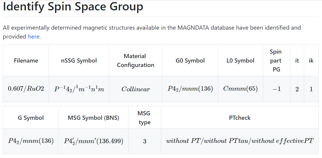
Fig. I3: The results of SSG identification, 151
All DFT calculations herein are performed using projector augmented wave
method, implemented in Vienna ab initio simulation package (VASP) [92, 93]. The
generalized gradient approximation of the Perdew-Burke-Ernzerhof-type exchange-
correlation potential [94] is adopted. To include the effect of electron correlation, the
DFT+U approach within the rotationally invariant formalism [95] were performing
with U eff = 2.0 eV for Ru 4d (RuO 2 ), U eff = 4.0 eV for Ce 4f (CeAuAl 3 ) and U eff = 1.0
eV for Co 3d (CoNb 3 S 6 ). Tight-binding models are constructed from DFT bands using
the WANNIER90 package [96, 97]; WannierTools package is used for the calculations
of anomalous hall conductivity [98].
152 References [1] M. S. Dresselhaus, G. Dresselhaus and A. Jorio, Group Theory: Application to the Physics of Condensed Matter, Springer (2008). [2] C. J. Bradley and A. P. Cracknell, The Mathematical Theory of Symmetry in Solids: Representation Theory for Point Groups and Space Groups, Oxford University Press (1972). [3] J. O. Dimmock, Use of Symmetry in the Determination of Magnetic Structures, Phys. Rev. 130, 1337 (1963). [4] H. M. Rietveld, A Profile Refinement Method for Nuclear and Magnetic Structures, J. Appl. Crystallogr. 2, 65 (1969). [5] H. Grimmer, Comments on tables of magnetic space groups, Acta Cryst. A 65, 145 (2009). [6] R.-J. Slager, A. Mesaros, V. Juričić and J. Zaanen, The space group classification of topological band-insulators, Nat. Phys. 9, 98 (2013). [7] J. Kruthoff, J. de Boer, J. van Wezel, C. L. Kane and R.-J. Slager, Topological Classification of Crystalline Insulators through Band Structure Combinatorics, Phys. Rev. X 7, 041069 (2017). [8] H. Watanabe, H. C. Po and A. Vishwanath, Structure and topology of band structures in the 1651 magnetic space groups, Sci. Adv. 4, eaat8685 (2018). [9] L. Elcoro, B. J. Wieder, Z. Song, Y. Xu, B. Bradlyn and B. A. Bernevig, Magnetic topological quantum chemistry, Nat. Commun. 12, 5965 (2021). [10] N. V. Belov and T. N. Tarkhova, Groups of colored symmetry, Sov. Phys. Crystallogr. 1, 5 (1956). [11] V. E. Naish, Magnetic structures of the metallic perovskites, Phys. Met. Metall. 14, 144 (1962). [12] V. E. Naish, On magnetic symmetry of crystals, Proc. USSR Acad. Sci. 27, 1496 (1963). [13] A. Kitz, Über die Symmetriegruppen von Spinverteilungen Von, Phys. Status Solidi B 10, 455 (1965). [14] W. F. Brinkman and R. J. Elliott, Theory of Spin-Space Groups, Proc. R. Soc. Lond. Ser. A 294, 343 (1966). [15] W. Brinkman and R. J. Elliott, Space Group Theory for Spin Waves, J. Appl. Phys. 37, 1457 (1966). [16] D. B. Litvin, Spin Translation Groups and Neutron Diffraction Analysis, Acta Cryst. A 29, 651 (1973). [17] D. B. Litvin and W. Opechowski, Spin Groups, Physica 76, 538 (1974). [18] D. B. Litvin, Spin Point Groups, Acta Cryst. A 33, 279 (1977). [19] P. F. Liu, J. Y. Li, J. Z. Han, X. G. Wan and Q. H. Liu, Spin-Group Symmetry in Magnetic Materials with Negligible Spin-Orbit Coupling, Phys. Rev. X 12, 021016 (2022). [20] A. Corticelli, R. Moessner and P. A. McClarty, Spin-space groups and magnon band topology, Phys. Rev. B 105, 064430 (2022). [21] L. Shekhtman, O. Entin-Wohlman and A. Aharony, Moriya's anisotropic superexchange interaction, frustration, and Dzyaloshinsky's weak ferromagnetism, 153 Phys. Rev. Lett. 69, 836 (1992). [22] B. A. Bernevig, J. Orenstein and S.-C. Zhang, Exact SU(2) Symmetry and Persistent Spin Helix in a Spin-Orbit Coupled System, Phys. Rev. Lett. 97, 236601 (2006). [23] J. Chaloupka and G. Khaliullin, Hidden symmetries of the extended KitaevHeisenberg model: Implications for the honeycomb-lattice iridates A 2 IrO 3 , Phys. Rev. B 92, 024413 (2015). [24] T. Jungwirth, X. Marti, P. Wadley and J. Wunderlich, Antiferromagnetic spintronics, Nat. Nanotechnol. 11, 231 (2016). [25] V. Baltz, A. Manchon, M. Tsoi, T. Moriyama, T. Ono and Y. Tserkovnyak, Antiferromagnetic spintronics, Rev. Mod. Phys. 90, 015005 (2018). [26] L. Šmejkal, Y. Mokrousov, B. Yan and A. H. MacDonald, Topological antiferromagnetic spintronics, Nat. Phys. 14, 242 (2018). [27] S. Hayami, Y. Yanagi and H. Kusunose, Momentum-Dependent Spin Splitting by Collinear Antiferromagnetic Ordering, J. Phys. Soc. Jpn. 88, 123702 (2019). [28] M. Naka, S. Hayami, H. Kusunose, Y. Yanagi, Y. Motome and H. Seo, Spin current generation in organic antiferromagnets, Nat. Commun. 10, 4305 (2019). [29] L. Šmejkal, R. Gonzalez-Hernandez, T. Jungwirth and J. Sinova, Crystal timereversal symmetry breaking and spontaneous Hall effect in collinear antiferromagnets, Sci. Adv. 6, eaaz8809 (2020). [30] S. Hayami, Y. Yanagi and H. Kusunose, Bottom-up design of spin-split and reshaped electronic band structures in antiferromagnets without spin-orbit coupling: Procedure on the basis of augmented multipoles, Phys. Rev. B 102, 144441 (2020). [31] I. I. Mazin, K. Koepernik, M. D. Johannes, R. Gonzalez-Hernandez and L. Šmejkal, Prediction of unconventional magnetism in doped FeSb 2 , Proc. Natl. Acad. Sci. 118 (2021). [32] L.-D. Yuan, Z. Wang, J.-W. Luo and A. Zunger, Prediction of low-Z collinear and noncollinear antiferromagnetic compounds having momentum-dependent spin splitting even without spin-orbit coupling, Phys. Rev. Mater. 5, 014409 (2021). [33] H. Y. Ma, M. Hu, N. Li, J. Liu, W. Yao, J. F. Jia and J. Liu, Multifunctional antiferromagnetic materials with giant piezomagnetism and noncollinear spin current, Nat. Commun. 12, 2846 (2021). [34] R. González-Hernández, L. Šmejkal, K. Výborný, Y. Yahagi, J. Sinova, T. Jungwirth and J. Železný, Efficient Electrical Spin Splitter Based on Nonrelativistic Collinear Antiferromagnetism, Phys. Rev. Lett. 126, 127701 (2021). [35] S. Karube, T. Tanaka, D. Sugawara, N. Kadoguchi, M. Kohda and J. Nitta, Observation of Spin-Splitter Torque in Collinear Antiferromagnetic RuO 2 , Phys. Rev. Lett. 129, 137201 (2022). [36] H. Bai, L. Han, X. Y. Feng, Y. J. Zhou, R. X. Su, Q. Wang, L. Y. Liao, W. X. Zhu,
Collinear Antiferromagnet RuO 2 , Phys. Rev. Lett. 128, 197202 (2022). [37] L. Šmejkal, A. B. Hellenes, R. González-Hernández, J. Sinova and T. Jungwirth, Giant and Tunneling Magnetoresistance in Unconventional Collinear Antiferromagnets with Nonrelativistic Spin-Momentum Coupling, Phys. Rev. X 12, 154 011028 (2022). [38] T. Berlijn, P. C. Snijders, O. Delaire, H. D. Zhou, T. A. Maier, H. B. Cao, S. X. Chi, M. Matsuda, Y. Wang, M. R. Koehler, P. R. C. Kent and H. H. Weitering, Itinerant Antiferromagnetism in RuO 2 , Phys. Rev. Lett. 118, 077201 (2017). [39] A. Bose, N. J. Schreiber, R. Jain, D.-F. Shao, H. P. Nair, J. Sun, X. S. Zhang, D. A. Muller, E. Y. Tsymbal, D. G. Schlom and D. C. Ralph, Tilted spin current generated by the collinear antiferromagnet ruthenium dioxide, Nat. Electron. 5, 267 (2022). [40] Z. Feng, X. Zhou, L. Šmejkal, L. Wu, Z. Zhu, H. Guo, R. González-Hernández, X. Wang, H. Yan, P. Qin, X. Zhang, H. Wu, H. Chen, Z. Meng, L. Liu, Z. Xia, J. Sinova, T. Jungwirth and Z. Liu, An anomalous Hall effect in altermagnetic ruthenium dioxide, Nat. Electron. 5, 735 (2022). [41] H. Bai, Y. C. Zhang, Y. J. Zhou, P. Chen, C. H. Wan, L. Han, W. X. Zhu, S. X. Liang, Y. C. Su, X. F. Han, F. Pan and C. Song, Efficient Spin-to-Charge Conversion via Altermagnetic Spin Splitting Effect in Antiferromagnet RuO 2 , Phys. Rev. Lett. 130, 216701 (2023). [42] D.-F. Shao, Y.-Y. Jiang, J. Ding, S.-H. Zhang, Z.-A. Wang, R.-C. Xiao, G. Gurung, W. J. Lu, Y. P. Sun and E. Y. Tsymbal, Néel Spin Currents in Antiferromagnets, Phys. Rev. Lett. 130, 216702 (2023). [43] D.-F. Shao, S.-H. Zhang, M. Li, C.-B. Eom and E. Y. Tsymbal, Spin-neutral currents for spintronics, Nat. Commun. 12, 7061 (2021). [44] Y.-P. Zhu, X. Chen, X.-R. Liu, Y. Liu, P. Liu, H. Zha, G. Qu, C. Hong, J. Li, Z. Jiang, X.-M. Ma, Y.-J. Hao, M.-Y. Zhu, W. Liu, M. Zeng, S. Jayaram, M. Lenger, J. Ding, S. Mo, K. Tanaka, M. Arita, Z. Liu, M. Ye, D. Shen, J. Wrachtrup, Y. Huang, R.- H. He, S. Qiao, Q. Liu and C. Liu, Observation of plaid-like spin splitting in a noncoplanar antiferromagnet, Nature 626, 523 (2024). [45] L. Šmejkal, J. Sinova and T. Jungwirth, Emerging Research Landscape of Altermagnetism, Phys. Rev. X 12, 040501 (2022). [46] L. Šmejkal, J. Sinova and T. Jungwirth, Beyond Conventional Ferromagnetism and Antiferromagnetism: A Phase with Nonrelativistic Spin and Crystal Rotation Symmetry, Phys. Rev. X 12, 031042 (2022). [47] S. Lee, S. Lee, S. Jung, J. Jung, D. Kim, Y. Lee, B. Seok, J. Kim, B. G. Park, L. Smejkal, C. J. Kang and C. Kim, Broken Kramers Degeneracy in Altermagnetic MnTe, Phys. Rev. Lett. 132, 036702 (2024). [48] J. Krempasky, L. Smejkal, S. W. D'Souza, M. Hajlaoui, G. Springholz, K. Uhlirova, F. Alarab, P. C. Constantinou, V. Strocov, D. Usanov, W. R. Pudelko, R. GonzalezHernandez, A. Birk Hellenes, Z. Jansa, H. Reichlova, Z. Soban, R. D. Gonzalez Betancourt, P. Wadley, J. Sinova, D. Kriegner, J. Minar, J. H. Dil and T. Jungwirth, Altermagnetic lifting of Kramers spin degeneracy, Nature 626, 517 (2024). [49] P. Liu, A. Zhang, J. Han and Q. Liu, Chiral Dirac-like fermion in spin-orbit-free antiferromagnetic semimetals, The Innovation 3, 100343 (2022). [50] Ao Zhang, Ke Deng, Jieming Sheng, Pengfei Liu, Shiv Kumar, Kenya Shimada, Zhicheng Jiang, Zhengtai Liu, Dawei Shen, Jiayu Li, Jun Ren, Le Wang, Liang Zhou, Yoshihisa Ishikawa, Takashi Ohhara, Qiang Zhang, Garry McIntyre, Dehong Yu, Enke Liu, Liusuo Wu, Chaoyu Chen and Q. Liu, Chiral Dirac fermion in a collinear 155
antiferromagnet, Chin. Phys. Lett. 40, 126101 (2023). [51] Jian Yang, Zheng-Xin Liu and C. Fang, Symmetry invariants in magnetically ordered systems having weak spin-orbit coupling, arXiv:2105.12738 (2021). [52] P.-J. Guo, Y.-W. Wei, K. Liu, Z.-X. Liu and Z.-Y. Lu, Eightfold Degenerate Fermions in Two Dimensions, Phys. Rev. Lett. 127, 176401 (2021). [53] L. M. Sandratskii, Symmetry analysis of electronic states for crystals with spiral magnetic order. I. General properties, J. Phys.: Condens. Matter 3, 8565 (1991). [54] L. M. Sandratskii, Symmetry analysis of electronic states for crystals with spiral magnetic order. II. Connection with limiting cases, J. Phys.: Condens. Matter 3, 8587 (1991). [55] N. Lazić, M. Milivojević and M. Damnjanović, Spin line groups, Acta Cryst. A 69, 611 (2013). [56] R. Lifshitz, Symmetry of magnetically ordered quasicrystals, Phys. Rev. Lett. 80, 2717 (1998). [57] R. Lifshitz and S. Even-Dar Mandel, Magnetically ordered quasicrystals: enumeration of spin groups and calculation of magnetic selection rules, Acta Cryst. A 60, 167 (2004). [58] S. Even-Dar Mandel and R. Lifshitz, Symmetry of magnetically ordered threedimensional octagonal quasicrystals, Acta Crystallogr A 60, 179 (2004). [59] https://findspingroup.com/. [60] S. V. Gallego, J. M. Perez-Mato, L. Elcoro, E. S. Tasci, R. M. Hanson, K. Momma, M. I. Aroyo and G. Madariaga, MAGNDATA: towards a database of magnetic structures. I. The commensurate case, J. Appl. Cryst. 49, 1750 (2016). [61] H. Wondratschek, General introduction to the subgroups of space groups, in: H. WondratschekandU. Müller (Eds.) International Tables for Crystallography Volume A1: Symmetry relations between space groups, Springer Netherlands (2004). [62] S. Ivantchev, E. Kroumova, J. Perez-Mato, J. Igartua, G. Madariaga and H. Wondratschek, SUPERGROUPS – a computer program for the determination of the supergroups of the space groups, J. Appl. Crystallogr. 35, 511 (2002). [63] L. Elcoro, B. Bradlyn, Z. Wang, M. G. Vergniory, J. Cano, C. Felser, B. A. Bernevig, D. Orobengoa, G. de la Flor and M. I. Aroyo, Double crystallographic groups and their representations on the Bilbao Crystallographic Server, J. Appl. Crystallogr. 50, 1457 (2017). [64] M. I. Aroyo, International Tables for Crystallography, Wiley Online Library (2013). [65] N. Belov, The 1651 shubnikov groups, Kristallografiya 2, 315 (1957). [66] A. V. Shubnikov, N. V. Belov and W. T. Holser, Colored symmetry, London: Pergamon Press (1964). [67] J. Q. Chen, M. J. Gao and G. Q. Ma, The Representation Group and Its Application To Space-Groups, Rev. Mod. Phys. 57, 211 (1985). [68] J.-Q. Chen, J. Ping and F. Wang, Group Representation Theory for Physicists, WORLD SCIENTIFIC (2002). [69] J. Li, Q. Yao, L. Wu, Z. Hu, B. Gao, X. Wan and Q. Liu, Designing light-element materials with large effective spin-orbit coupling, Nat. Commun. 13, 919 (2022).
156 [70] I. T. Atsushi Togo, Spglib: a software library for crystal symmetry search, arXiv:1808.01590 (2018). [71] S. P. Ong, W. D. Richards, A. Jain, G. Hautier, M. Kocher, S. Cholia, D. Gunter, V.
robust, open-source python library for materials analysis, Comput. Mater. Sci. 68, 314 (2013). [72] D. T. Adroja, C. de la Fuente, A. Fraile, A. D. Hillier, A. Daoud-Aladine, W. Kockelmann, J. W. Taylor, M. M. Koza, E. Burzurí, F. Luis, J. I. Arnaudas and A. del Moral, Muon spin rotation and neutron scattering study of the noncentrosymmetric tetragonal compound CeAuAl 3 , Phys. Rev. B 91, 134425 (2015). [73] L.-D. Yuan, Z. Wang, J.-W. Luo, E. I. Rashba and A. Zunger, Giant momentumdependent spin splitting in centrosymmetric low-Z antiferromagnets, Phys. Rev. B 102, 014422 (2020). [74] N. J. Ghimire, A. S. Botana, J. S. Jiang, J. Zhang, Y. S. Chen and J. F. Mitchell, Large anomalous Hall effect in the chiral-lattice antiferromagnet CoNb 3 S 6 , Nat. Commun. 9, 3280 (2018). [75] G. Tenasini, E. Martino, N. Ubrig, N. J. Ghimire, H. Berger, O. Zaharko, F. Wu, J. F. Mitchell, I. Martin, L. Forró and A. F. Morpurgo, Giant anomalous Hall effect in quasi-two-dimensional layered antiferromagnet Co 1/3 NbS 2 , Phys. Rev. Res. 2, 023051 (2020). [76] H. Tanaka, S. Okazaki, K. Kuroda, R. Noguchi, Y. Arai, S. Minami, S. Ideta, K. Tanaka, D. Lu, M. Hashimoto, V. Kandyba, M. Cattelan, A. Barinov, T. Muro, T. Sasagawa and T. Kondo, Large anomalous Hall effect induced by weak ferromagnetism in the noncentrosymmetric antiferromagnet CoNb 3 S 6 , Phys. Rev. B 105, L121102 (2022). [77] X. P. Yang, H. LaBollita, Z.-J. Cheng, H. Bhandari, T. A. Cochran, J.-X. Yin, M. S. Hossain, I. Belopolski, Q. Zhang, Y. Jiang, N. Shumiya, D. Multer, M. Liskevich, D. A. Usanov, Y. Dang, V. N. Strocov, A. V. Davydov, N. J. Ghimire, A. S. Botana and M. Z. Hasan, Visualizing the out-of-plane electronic dispersions in an intercalated transition metal dichalcogenide, Phys. Rev. B 105, L121107 (2022). [78] H. Takagi, R. Takagi, S. Minami, T. Nomoto, K. Ohishi, M. T. Suzuki, Y. Yanagi, M. Hirayama, N. D. Khanh, K. Karube, H. Saito, D. Hashizume, R. Kiyanagi, Y. Tokura, R. Arita, T. Nakajima and S. Seki, Spontaneous topological Hall effect induced by noncoplanar antiferromagnetic order in intercalated van der Waals materials, Nat. Phys. 19, 961 (2023). [79] S. S. P. Parkin, E. A. Marseglia and P. J. Brown, Magnetic structure of Co 1/3 NbS 2 and Co 1/3 TaS 2 , J. Phys. C: Solid State Phys. 16, 2765 (1983). [80] N. Nagaosa, J. Sinova, S. Onoda, A. H. MacDonald and N. P. Ong, Anomalous Hall effect, Rev. Mod. Phys. 82, 1539 (2010). [81] R. Shindou and N. Nagaosa, Orbital Ferromagnetism and Anomalous Hall Effect in Antiferromagnets on the Distorted fcc Lattice, Phys. Rev. Lett. 87, 116801 (2001). [82] M. Hirschberger, Y. Nomura, H. Mitamura, A. Miyake, T. Koretsune, Y. Kaneko,
Geometrical Hall effect and momentum-space Berry curvature from spin-reversed band 157 pairs, Phys. Rev. B 103, L041111 (2021). [83] L. Šmejkal, A. H. MacDonald, J. Sinova, S. Nakatsuji and T. Jungwirth, Anomalous Hall antiferromagnets, Nat. Rev. Mater. 7, 482 (2022). [84] Yi Jiang, Ziyin Song, Tiannian Zhu, Zhong Fang, Hongming Weng, Zheng-Xin Liu, Jian Yang and C. Fang, Enumeration of spin-space groups: Towards a complete description of symmetries of magnetic orders, arXiv:2307.10371 (2023). [85] Zhenyu Xiao, Jianzhou Zhao, Yanqi Li, Ryuichi Shindou and Z.-D. Song, Spin Space Groups: Full Classification and Applications, arXiv:2307.10364 (2023). [86] K. Shinohara, A. Togo, H. Watanabe, T. Nomoto, I. Tanaka and R. Arita, Algorithm for spin symmetry operation search, Acta Cryst. A 80, 94-103 (2024). [87] H. Watanabe, K. Shinohara, T. Nomoto, A. Togo and R. Arita, Symmetry analysis with spin crystallographic groups: Disentangling effects free of spin-orbit coupling in emergent electromagnetism, Phys. Rev. B 109, 094438 (2024). [88] Hana Schiff, Alberto Corticelli, Afonso Guerreiro, Judit Romhányi and P. McClarty, The Spin Point Groups and their Representations, arXiv:2307.12784 (2023). [89] M. I. Aroyo, J. M. Perez-Mato, C. Capillas, E. Kroumova, S. Ivantchev, G. Madariaga, A. Kirov and H. Wondratschek, Bilbao Crystallographic Server: I. Databases and crystallographic computing programs, Z. Kristallogr. Cryst. Mater. 221, 15 (2006). [90] J. Yang and Z.-X. Liu, Irreducible projective representations and their physical applications, J. Phys. A: Math. Theor. 51, 025207 (2017). [91] Y. Xu, L. Elcoro, Z.-D. Song, B. J. Wieder, M. G. Vergniory, N. Regnault, Y. Chen,
materials, Nature 586, 702 (2020). [92] G. Kresse and J. Furthmüller, Efficient iterative schemes for ab initio total-energy calculations using a plane-wave basis set, Phys. Rev. B 54, 11169 (1996). [93] G. Kresse and D. Joubert, From ultrasoft pseudopotentials to the projector augmented-wave method, Phys. Rev. B 59, 1758 (1999). [94] J. P. Perdew, K. Burke and M. Ernzerhof, Generalized Gradient Approximation Made Simple, Phys. Rev. Lett. 77, 3865 (1996). [95] S. L. Dudarev, G. A. Botton, S. Y. Savrasov, C. J. Humphreys and A. P. Sutton, Electron-energy-loss spectra and the structural stability of nickel oxide: An LSDA+U study, Phys. Rev. B 57, 1505 (1998). [96] A. A. Mostofi, J. R. Yates, Y.-S. Lee, I. Souza, D. Vanderbilt and N. Marzari, wannier90: A tool for obtaining maximally-localised Wannier functions, Comput. Phys. Commun. 178, 685 (2008). [97] N. Marzari, A. A. Mostofi, J. R. Yates, I. Souza and D. Vanderbilt, Maximally localized Wannier functions: Theory and applications, Rev. Mod. Phys. 84, 1419 (2012). [98] Q. Wu, S. Zhang, H.-F. Song, M. Troyer and A. A. Soluyanov, WannierTools: An open-source software package for novel topological materials, Comput. Phys. Commun. 224, 405 (2018).
158