
⬇ Download Markdown · ⬇ Download LaTeX · ⬇ original · view original
1 Dartmouth College, NH, USA ¶ Corresponding author DOI: 10.21105/joss.06644 Software
• Review • Repository • Archive Editor: Johanna Bayer Reviewers:
• @thelfer • @svenweihe • @imperialiluc
Submitted: 20 December 2023 Published: 02 September 2025 License Authors of papers retain copyright and release the work under a Creative Commons Attribution 4.0 International License (CC BY 4.0).
The partial element equivalent circuit method (PEEC) is a particularly interesting integralequation method for electromagnetic problems as it can be easily combined with circuit simulations and does not require a discretization of the free space. This paper introduces PyPEEC, an open-source Python solver targeting 3D quasi-magnetostatic problems such as inductors, transformers, chokes, IPT coils, or busbars. The geometry is described with voxels and the solver uses an FFT-accelerated variant of the PEEC method. The FFT acceleration drastically reduces the computational cost and the memory footprint.
Quasi-magnetostatic field simulations are widely used for the design and optimization of electrical components (e.g., power electronics, packaging, IC design). Among the existing numerical methods (e.g., FEM, FDTD, PEEC, BEM), the PEEC method features several advantages (Jithesh & Pande, 2003; A. Ruehli et al., 2017; A. E. Ruehli, 1974; Torchio, 2019):
• Only the active materials are discretized (no need to mesh the vacuum/air). • Intuitive understanding of the equation discretization process. • Straightforward connection of external circuit elements. The fundamental drawback of the classical PEEC method is that the matrix describing the equation system is not sparse. This means that the computational cost and the memory requirement become problematic for large problems. This problem can be mitigated if the geometry is represented with voxels (Torchio, Lucchini, et al., 2022; A. C. Yucel et al., 2018). The first advantage of such geometries is that the Green’s functions (i.e., the inductance and potential matrices) have analytical solutions, avoiding computationally intensive numerical integrals (Hoer & Love, 1965; Piatek & Baron, 2012). The second advantage is that, due to the regular voxel discretization, many coefficients of the inductance and potential matrices are redundant. The dense matrices are block-Toeplitz Toeplitz-block matrices and feature the following key properties (Lee, 1986; Polimeridis et al., 2014):
• The block-Toeplitz Toeplitz-block matrices can be embedded into circulant tensors,
reducing the memory requirements from 𝑂(𝑛 2 ) to 𝑂(𝑛) . • The matrix-vector multiplications can be done with Fourier transforms. With an FFT
algorithm, the computational complexity of matrix-vector multiplications is reduced from
Guillod, & Sullivan. (2025). PyPEEC: A 3D Quasi-Magnetostatic Solver using an FFT-Accelerated PEEC Method with Voxelization. Journal of 1 Open Source Software , 10 (113), 6644. https://doi.org/10.21105/joss.06644.

Different variants of the FFT-accelerated PEEC method have been shown to be extremely fast for a large variety of electromagnetic problems, such as high-frequency transformers (Torchio, Lucchini, et al., 2022), power inductors (Marconato & Lucchini, 2021), human body field exposure (Torchio, Arduino, et al., 2022), nuclear fusion devices (Bettini et al., 2020), and PCB layouts (Romano et al., 2023). An open-source implementation (“FFT-PEEC”) of the FFT-accelerated PEEC method already exists (Torchio & Lucchini, 2020, 2021). However, this code can only handle magnetic materials for static simulations (and not in the frequency domain). Moreover, depending on the considered quasi-static problem (e.g., geometries with multiple conductors), the source code requires some adaptations. The open-source tools “VoxHenry” and “MARIE” are also using FFT-accelerated methods, but are specialized for full-wave solutions without magnetic materials (Villena et al., 2015; A. Yucel, 2018). Finally, it should be noted that all the aforementioned implementations depend on proprietary programming languages and libraries. PyPEEC, the tool introduced in this paper, addresses these needs by providing a 3D quasimagnetostatic implementation of the FFT-accelerated PEEC method (Torchio, Lucchini, et al., 2022). PyPEEC is a fully open-source (MPL 2.0 licence and implemented in Python) and offers a general-purpose solver by allowing the description of arbitrary problems without having to modify the source code.
In this paper, the release 5.7 of PyPEEC is considered. PyPEEC solves 3D magnetostatic and quasi-magnetostatic problems with voxel geometries. An arbitrary number of conductive domains, magnetic domains (ideal and/or lossy), and sources (voltage and/or current) can be used. The current density, flux density, electric potential, magnetic potential, and loss density are computed. The free space magnetic field (near-field) can also be computed on a point cloud. Additionally, the voltage, current, complex power, and impedance of the different terminals are extracted.
Description of the geometry Description of the voxel structure Description of the quasi-static problem Description of the solver num. tolerance mesher - Create the geometry solver - Solve the PEEC problem Voxelization of the geometry
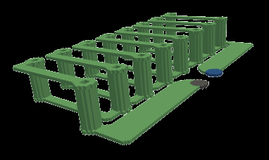
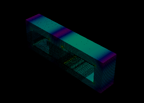
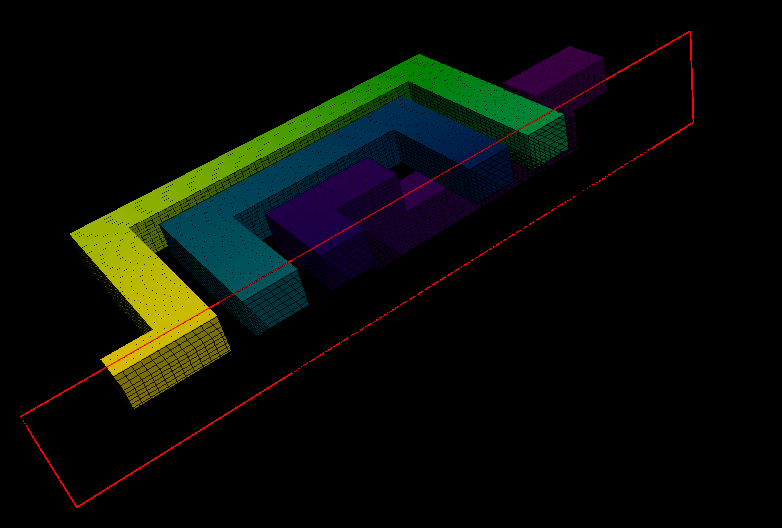
Using 3D STL files Using 2D vector shapes (layer stack) Using PNG files (layer stack) Using GERBER files (layer stack) Using voxel index vectors Resolve conflicts between domains Refine and/or resample the voxels Compute the connected components Check the domain connections Compute the incidence matrices Post-process the solution (field, power, etc.)


Guillod, & Sullivan. (2025). PyPEEC: A 3D Quasi-Magnetostatic Solver using an FFT-Accelerated PEEC Method with Voxelization. Journal of 2 Open Source Software , 10 (113), 6644. https://doi.org/10.21105/joss.06644.

PyPEEC is implemented in pure Python using NumPy, SciPy, Joblib, Rasterio, Shapely, Pillow, Matplotlib, and PyVista. The solver is able to leverage multi-core CPUs and GPUs. Optional HPC libraries are available for accelerating the sparse preconditioner factorization (MKL/PARDISO and PyAMG) and the FFT operations (FFTW, MKL/FFT, and CuPy/CUDA). PyPEEC can be used through an API, a command-line tool, or Jupyter notebooks. The package is available through the Python package index (PyPi) and the community-driven Conda package index (conda-forge). A Docker image with JupyterLab is also maintained. Figure 1 depicts the PyPEEC workflow. First, the mesher builds the geometry (from vector shapes, STL files, PNG files, or GERBER files), performs the voxelization, and checks the validity of the discretization. Afterward, the solver creates the FFT-multiplication operators, assembles the equation systems, extracts sparse preconditioners, solves the problem, and post-processes the solution. The viewer and the plotter are used to visualize the results. Alternatively, ParaView can be used to analyze and visualize the solutions.
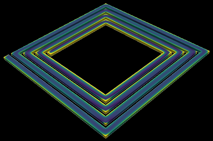
To demonstrate the performance of the solver, a planar air-core spiral inductor is considered (Guillod & Sullivan, 2025). The inductor has a footprint of 4 mm 2 and is operated in the 40.68 MHz ISM band. Figure 2 shows the ratio between the AC and DC current densities, the relative error on the extracted impedance, and the computational cost. The number of degrees of freedom represents the number of unknowns for the PEEC problem (dense equation system). The computational cost is evaluated with an AMD EPYC 7543 CPU (without GPUs).
(a) (b) (c)
Figure 2: (a) Ratio between the AC and DC current densities. (b) Relative error on the extracted equivalent resistance and the inductance. (c) Wall clock time duration for the complete workflow.
As the skin depth is smaller than the dimension of the conductor, the eddy currents are non-negligible. This implies that, with a coarse discretization, the resistance value is less accurate than the inductance value. With a tolerance of 4%, the quasi-static problem is solved in 4 seconds. The FFT acceleration allows dense PEEC problems with 10 7 degrees of freedom to be solved in 80 seconds. The performances of PyPEEC are impacted by the following factors. For problems dominated by eddy currents and/or containing magnetic materials, the majority of the computational effort (typically over 70%) is linked to the FFT-accelerated multiplications. In such cases, the performances are directly driven by the FFT solver and benefit from the available parallel and GPU algorithms. Finally, it should be noted that PyPEEC is using a regular voxel structure to represent the geometry. This implies that large geometries with small features cannot be meshed efficiently.
Guillod, & Sullivan. (2025). PyPEEC: A 3D Quasi-Magnetostatic Solver using an FFT-Accelerated PEEC Method with Voxelization. Journal of 3 Open Source Software , 10 (113), 6644. https://doi.org/10.21105/joss.06644.

This work was supported by the Power Management Integration Center (NSF IUCRC) at Dartmouth College under Grant No. PMIC-062. The authors would like to thank Yue (Will) Wu for discovering and reporting several bugs.
Bettini, P., Torchio, R., Lucchini, F., Voltolina, D., & Alotto, P. (2020). Fast Fourier
Transform-Volume Integral: a Smart Approach for the Electromagnetic Design of Complex Systems in Large Fusion Devices. Plasma Physics and Controlled Fusion, 63(2), 025010. https://doi.org/10.1088/1361-6587/abce8f Guillod, T., & Sullivan, C. R. (2025). Free-Shape Optimization of VHF Air-Core Inductors
using a Constraint-Aware Genetic Algorithm. Proc. Of the Applied Power Electronics Conf. And Expo. (APEC), 1–8. https://doi.org/10.1109/APEC48143.2025.10977326 Hoer, C., & Love, Y. (1965). Exact Inductance Equations for Rectangular Conductors with
Applications to more Complicated Geometries. Journal of Research of the National Bureau of Standards, 69(2), 127–137. https://doi.org/10.6028/jres.069c.016 Jithesh, V., & Pande, D. C. (2003). A Review on Computational EMI Modelling Techniques.
Proc. Of the Int. Conf. On Electromagnetic Interference and Compatibility (INCEMIC), 159–166. https://doi.org/10.1109/ICEMIC.2003.1287800 Lee, D. (1986). Fast Multiplication of a Recursive Block Toeplitz Matrix by a Vector and its Ap-
plication. Journal of Complexity, 2(4), 295–305. https://doi.org/10.1016/0885-064X(86) 90007-5 Marconato, N., & Lucchini, F. (2021). Application of FFT-PEEC Method for Nonlinear
Inductance Extraction. Proc. Of the Int. Conf. On Electrical, Computer, Communications and Mechatronics Engineering (ICECCME), 1–6. https://doi.org/10.1109/ICECCME52200. 2021.9590864 Piatek, Z., & Baron, B. (2012). Exact Closed Form Formula for Self Inductance of Conductor
of Rectangular Cross Section. Progress In Electromagnetics Research, 26, 225–236. https: //doi.org/10.2528/PIERM12080314 Polimeridis, A. G., Villena, J. F., Daniel, L., & White, J. K. (2014). Stable FFT-JVIE Solvers
for Fast Analysis of Highly Inhomogeneous Dielectric Objects. Journal of Computational Physics, 269, 280–296. https://doi.org/10.1016/j.jcp.2014.03.026 Romano, D., Kovacevic-Badstuebner, I., Antonini, G., & Grossner, U. (2023). Efficient PEEC
Iterative Solver for Power Electronic Applications. IEEE Transactions on Electromagnetic Compatibility, 65(2), 546–554. https://doi.org/10.1109/TEMC.2023.3238394 Ruehli, A. E. (1974). Equivalent Circuit Models for Three-Dimensional Multiconductor
Systems. IEEE Transactions on Microwave Theory and Techniques, 22(3), 216–221. https://doi.org/10.1109/TMTT.1974.1128204 Ruehli, A., Antonini, G., & Jiang, L. (2017). Circuit Oriented Electromagnetic Modeling Using
the PEEC Techniques. Wiley. https://doi.org/10.1002/9781119078388 Torchio, R. (2019). A Volume PEEC Formulation Based on the Cell Method for Electromagnetic
Problems From Low to High Frequency. IEEE Transactions on Antennas and Propagation, 67 (12), 7452–7465. https://doi.org/10.1109/TAP.2019.2927789 Guillod, & Sullivan. (2025). PyPEEC: A 3D Quasi-Magnetostatic Solver using an FFT-Accelerated PEEC Method with Voxelization. Journal of 4 Open Source Software , 10 (113), 6644. https://doi.org/10.21105/joss.06644.

Torchio, R., Arduino, A., Zilberti, L., & Bottausci, O. (2022). A Fast Tool for the Parametric
Analysis of Human Body Exposed to LF Electromagnetic Fields in Biomedical Applications. Computer Methods and Programs in Biomedicine, 214, 106543. https://doi.org/10.1016/j. cmpb.2021.106543 Torchio, R., Lucchini, F., Schanen, J. L., Chadebec, O., & Meunier, G. (2022). FFT-PEEC:
A Fast Tool From CAD to Power Electronics Simulations. IEEE Transactions on Power Electronics, 37 (1), 700–713. https://doi.org/10.1109/TPEL.2021.3092431 Torchio, R., & Lucchini, L. (2020). FFT-PEEC. In GitHub repository. GitHub. https:
//github.com/UniPD-DII-ETCOMP/FFT-PEEC Torchio, R., & Lucchini, L. (2021). FFT-NLIE. In GitHub repository. GitHub. https:
//github.com/UniPD-DII-ETCOMP/FFT-NLIE Villena, J. F., Polimeridis, A., & Serralles, J. (2015). MARIE. In GitHub repository. GitHub.
https://github.com/thanospol/MARIE Yucel, A. (2018). VoxHenry. In GitHub repository. GitHub. https://github.com/acyucel/
VoxHenry Yucel, A. C., Georgakis, I. P., Polimeridis, A. G., Bagci, H., & White, J. K. (2018). VoxHenry:
FFT-Accelerated Inductance Extraction for Voxelized Geometries. IEEE Transactions on Microwave Theory and Techniques, 66(4), 1723–1735. https://doi.org/10.1109/TMTT. 2017.2785842 Guillod, & Sullivan. (2025). PyPEEC: A 3D Quasi-Magnetostatic Solver using an FFT-Accelerated PEEC Method with Voxelization. Journal of 5 Open Source Software , 10 (113), 6644. https://doi.org/10.21105/joss.06644.