
⬇ Download Markdown · ⬇ Download LaTeX · ⬇ original · view original · CSV: table 1, table 2



A Data Distributed,

Ma +> J ames h;. Painter:,
NASA

tDepart.ment 5 Advanced Algorithm Mail Kwan-Lirr
tlCASE, Parallel C:onlputing Stop 1:32C, C:harles Langley of Computer Science, Laboratory, Los Alanlos

kmaUicasc.edu, for Ray-Traced Iiniversity j~nie(~~cs.utall.edu,






2

















o 1993 Lake City,
Virginia 231X1
I.!tah 84112 Los Alamos, New Mexico 87545 kroghWacl.lanl.gov Related Work An increasing nunlber of parallel architectures and algorithrns for volunle rendering have been developed. The niajor algorithxnic strategy for parallelizing volume rendering is the divide-and-conquer paradigni. The volu~nc rendering probleni can be subdivided either in data space or in image space. While data-space subdivision assigns the conlputation associated with particular subvolurnes to processors, image-space subdivision distributes t,he computation rr<sociated with particular portions of t.he image space. Data-space subdivision is usually applied to a distributed-nlelnory parOn the other hand. iniage- allel computing environnlent. space snbdivision is sitnple and efficient for shared-rnenlory mult.iprocessing. Ilybrid methods are also feasible.
Anlong the parallel architectures developed which are capable of perforlning interactive volunle rendering, the F’ixelPlanes 5 systenl [s] is a heterogeneous nlultiprocessor graphics systeni using both MIMI) and SIM 11 parallelisnl. The hardware consists of uiultiple i86O-based Graphics Processors? multiple SIMD pixel-processors arrays called Kenderers, and a conventional 1380x1024-pixel franle buffer, interconnected by a five-gigabit ring network. In [Z3], variations of parallel volurne rendering irnplernented on t.his systein are presented. One approach similar to the idea we proposed earlier in [II] and now elaborate in this paper, distributes data as well as ray casting anlong separate Graphics Processors and reconstructs the ray segnients into coherent rays. Incorporating dynamic load balancing, lookup tables and progressive refineulent, this approach can render shaded inages froui 128 x 1’28 x 56 volunie data at 20 fralnes per second. In the following sect.ions, we survey most recent research results front other algorithnlic approaches.
NetExisting volurne rendering tnethods, though capable of rnaking very effective visualizations, are very coniputationally intensive and therefore fail to achieve interactive rendering by the rates for large data sets. Our work was nlotivated following ob$ervations: First, volunle data sets can be quite large, often too large for a single workstation to hold in ineinory at once. Moreover, high quality volunie reuderings norlnally take tninutes to hours on a single processor uiachine and the rendering time usually grows linearly with the data size. To achieve.interactive rendering rates, users often nlust reduce the original data, which produces poor visualization results. Second, many acceleration techniques and data exploration techniques for volume rendering trade rnernory for time. Third, rnotion is one of the nlost effective visualization techniques. An anirnation sequence of volulnc visualization normally takes hours to days to generate. Finally, we notice the availability of hundreds of high perfornuance workstations in our computing environlnent, which are frequently sitting idle for nlany hours a day. This lead us to consider ways to distribute the increasing axnount of data as well as the tinle-consuming rendering process to the tremendous distributed conlputing resources available to us.
In this paper, we describe the resulting parallel votunle rendering algorithm and a image cornpositing method along with their iniplernentations and perforniance on the C:M-5 and networked workstations. For a homogeneous computing environnient, a conlputing environment with uniformly distributed processing and nlelnory units, this parallel volume $3.00 Laboratory, 5, Michael Hampton, Rendering rendering algorithrn evenly distributes data to the conlputing resources available. Each subvolume is then ray-traced locally and generates a partial iinage, without, the need to cornrnunicate with other processing units. These partial iniages are nierged in the proper order through a new parallel cornpositing algorithni to achieve the correct final image. Our test results on both the honlogeneous and heterogeneous computing environments are promising, and expose different performance tuning issues for each environment.
Introduction O-81 86-4920.8/93 Salt ha~~sel~!~~acl.lalll.gov, This paper presents a divide-and-conquer ray-traced volulne rendering algorithrn and a parallel inlage cornpositing nlethod, along with their implenlentation and perforinance on the (-:onnection Machine (‘:IM-. and networked workstations. This algorithm distributes 1ot.h the data and the conlputations to individual processing units to achieve fast, high-quality rendering of high-resolution data. The volume data, once distributed, is left intact. The processing nodes perforni local raytracing of their subvolulne concurrently. No coniluunication between processing units is needed cluring this locally ray-tracing process. A subiruage is generated by each processing unit and the final inlage is obtained by cornpositing subiniages in the proper order, which can be deterrnined a priori. Test results on the C:M-5 and a group of networked workstations denlonstrate the practicality of our rendering algorithrn and conlpositing method. . , 1 Center, of 1!tah, National Abstract Key Words: Scientific Visualization, Volunle Rendering, work CZoniputing, Massively Parallel F’rocessing.
1). Hansen Research Volume 2.1 Montani
Montani et nl. [13] propose a hybrid ray-traced ncthod for running on distributed-melnory parallel systenls like a n(-:UBE, in which processing nodes are organized into a set of clu.ste each of them composed of the same nurnbcr of nodes. The ilnagc space is partitioned and a subset of pixels is assigned to each cluster, which will colnpute pixel values IEEE

15




independently. Data to be visualized is replicated in each cluster, and is partitioned among the local memory of the cluster’s nodes. A static load balancing strategy based on

the estimated work load of each processor is used to improve efficiency, and on average a twenty percent speedup in ren-

dering time can be obtained. In addition, a mechanism for preventing deadlock is necessary to handle the dependency bctwcen processing nodes in the same cluster. The best cf-

ficiency reported by the authors while using a single cluster of 128 nodes is 0.74. However, when increasing the number

of clusters, the efficiency drops significantly. For example, using 16 clusters with 8 nodes per cluster, the efficiency re-

ported is only 0.31.
Smith [2], and Hanrahan [7], converts both 3D rotation and perspective transformations into only four 1 D shear/scale passes, compared to Schrijder’s eight-pass rotation algorithm composed exclusively of shear operations. Volume transposition is then performed to localize data access. MP-1 provides a global router which allows efficient moving of data between F’Es. On a 16K-PE MP-1, a 128x128-pixel volume rendered image of a 1283-voxel data can be generated in snbseconds. However, it seems that if either a smaller number of PEs or larger data sets arc used, the data transposition time can degrade the performance significantly.
2.2 The idea behind our algorithm is very simple: divide the

data up into smaller subvolumes distributed to multiple computers, render them separately and locally, and combine

the resulting images in an incremental fashion. While multiple computers are available, the memory demands on each computer are modest since each computer need only hold a

subset of the total data set. This approach can be used t,o render high resolution data sets in an environment, for exam-

ple, with many midrange workstations (e.g. equipped with 16MR memory) on a local area network. Many computing

environments have an abundance of such workstations which could be harnessed for volume rendering provided that the memory usage on each machine is reasonable.
3
Nieh
Nieh and Levoy [14] implement ray-traced volume rendering on Stanford DASH Multiprocessors, a scalable sharedmemory MIMD machine. Their method employs algorithmic opiimizations such as hierarchical opacity enumeration, early ray termination, and adaptive image sampling [9]. The shared-memory architecture providing a single address space The parallel al- allows straightforward implementations. gorithm distributes volume data in an interleaved fashion among the local memories to avoid hot spotting. The ray tracing computation is distributed among the processors by partitioning the image plane into contiguous blocks and each

processor is st.atically assigned an image block. Each block is further divided into square image tiles for load balancing purposes. When a processor is done computing its block,

instead of waiting, it steals tiles from a neighboring processor’s block to keep itself busy. Experiment results show

this load balancing scheme cuts the variation of execution times across the 48 processors used by 90%. Currently, each processor in DASH is a 33 MHz MIPS RBOOO. IJsing all

48 processors available, a 416x416-pixel image for a 256” data set can be generated in subsections; for nonadaptive

sampling, the speedup over uniprocessor rendering is 40.

2.3 3.1 Ray-Traced Volume Algorithm Rendering
The st,arting point of our algorithm is the volume ray-tracing technialue presented by Levoy [8]. A n image is constructed in image orcl~r by casting rays from the eye through the image plane aud into the volume of data. One ray per pixel is generally sufficient, provided that the image sample density is higher than the volume data sample density. Using a discret,e rendering model, the data volume is sampled at evenly spaced points along the ray, usually at a rate of one to two samples per voxel. At each sample point on the ray, a color and an opacity are computed using trilinear interpolation from the data values at each of the eight nearest voxcls.
The color is assigned by applying a shading function such

as the F’hong lighting model. A color map is often used to assign colors to the raw data values. The normalized gra-

dient of the data volume can be used as the surface normal for shading calculations. The opacity is derived by using the interpolated voxel values as indices into an opacity map.

Sampling continues until the data volume is exhausted or until the accumulated opacity reaches a threshold cut.-off

value. The final image value corresponding to each ray is formed by compositing, front-to-back. the colors and opacities of the sample point.s along the ray. The color/opacity

compositing is based on Porter and Duff’s over operator [16]. It is easy to verify that the over is nssociatiuc; that is, Schriider
Schriider and Stall [18] develop a data-parallel ray-traced volume rendering algorithm that exploits ray parallelism. They describe the ray tracing steps as discrete line drawing. This algorithm is both more memory efficient and less communications bound than an algorithm introduced earlier by the first author [I?‘]. They have implemented this algorithm on both the Connection Machine CM-2 and the Princeton Engine, which consists of 2048 Is-bit DSP processors arranged in a ring. To allow for a SIMD implementation, rays initially enter only the front-most face of the volume and proceed in lock step. Consequently, each sample has the same local coordinates in a voxel. When rays exit the far face, a toroidal shift of the data is performed and new rays are initialized to enter the visible side face of the volume. As

a result, the rotation angle selected influences about 10% of the runtime of the algorithm. Tests using a 128’-voxel data

set on both the CM2 from 8K to 32li processors in size and the F’rinceton Engine of 1024 processors show subsecond rendering time.

2.4 A Divide-and-Conquer a over (b over c) = (a over h) over C.
The associativity of the over operator allows us t,o break a ray up into segments, process the sampling and composit.ing of each segment independently, and combine the results from each segment via a final compositing step. This is the basis for our parallel volume rendering algorithm. Vdzina

VCzina. et al. [21] implement a multi-pass algorithm similar to Schriider’s on MP-1, which is a massively data-parallel

SIMD computer with a 2D array of processing elements ([‘Es). Their algorithm, based on work done by (fatmull and 3.2 Data Subdivision/Load Balancing
The divide-and-conquer algorithm requires that we partition the input data into subvolumcs. There are many ways


16




k k+l n




Boundary Replication.
Subvolume Figure 2: Volume


Subvolume

Figure 1: k-Dtree Subdivision of a Data 2 Volume


to partition the data; the only requirement is that an unaubiuous front,-to-back ordering can be determined for the subvolumes to establish the required order for corupositing

subimages. Ideally we would like each subvolume to require about the same amount of computation. In practice, this

is gener,ally not something that we can always control well. For example, if the viewpoint is known and fixed, we could partition the volume in a manner that minimizes the overlap

betweeu the images resulting from the subvolumes. This will reduce the cost of the merging since cornpositing need only

be applied where subimages overlap as shown later. For an auiulation sequence, this technique can not be applied since the viewpoint changes with each frame. We can also parti-

tion the volume based on an estimation of the distribution of the amount of computation within the volume by pre-

processing the volume to identify high gradient regions or empty regions. In addition, we may partition and distribute the volume according to the performance of individual conl-

put,ers when using a heterogeneous computing environment.
The simplest method is probablv to partition the voluruc

along planes parallel to the coordinate planes of the data. Again, if the viewpoint is fixed and known when partition-

ing the data, the coordinate plane most nearly orthogonal to the view direction can be determined and the data can subdivided into “slices” orthogonal to this plane. When ortho-

graphic projection is used, this will tend to produce subimages with littlc overlap. If the view point is not known,

or if perspective projection is used, it is better to partition the volume equally along ~11 coordinate planes. This can be accomplished using a k-.D tree structure [l], with alternat-

ing binary subdivision of the coordinate planes at each level in the tree m indicated in Figure 1. As shown later, this

structure provides a nice mechanism for image cornpositing.
As shown in Figure 2, when a volu~ue of grid points (vox-

els) is evenly subdivided into, for example! two subvolumes, each subvolume may contain half of the total grid points. Note that each voxcl is located at a corner of the grid. Con-

sequently, those ray samples that lie in the cut boundary region (the dotted region) are lost. If the view vector is

parallel to the cut plane, a black strip will appear at each cut boundary in the composited image. In order to avoid this problem, we need to replicate one layer of the bound-

ary grid at each subvolurne so the composited ray-casting image does not drop out features originally in the volume. is For the cast shown in Figure 2, one possible arrangement Figure 3: Correct that Subvolume 2 includes layer k is replicated.
I includes k to layer 3.3 Rendering Parallel Ray Sampling.
layer 1 to layer k and Subvolume II; that is, in Subvoluule 2, layer We USC ray-casting based volr~~nc rendering. Each computer can perform raytracing independently; that is, there is no data conmiunication rdquired during the subvolume rendering. All subvolumes are rendered using an ideutical view position and only rays within the image region covering the corresponding subvolume are cast and sampled. Since we sample along each ray at a predetermined interval! cousistent sampling locations must be ensured for all subvolumcs so we can reconstruct the original volume. As shown in Figure 3, for example, the location of the first sample ,$(I) on the ray shown in Subvolume 2 should be calculated correct.ly so that the distance between $(l) and .41(n) is equivalent. to the predetermined interval. Otherwise, mall features in the data might be lost or enhanced in an erroneous way.
3.4 Image Composition
The final step of our algorithm is to merge ray segmeuts and thus all partial images into the final total image. In order to merge, we need t.o store uot only the color at. each pixel but also the accumulated opacity there. As described earlier, the rule for merging subimages is based ou the river corn-- positing operator. iVhen all subimages are ready, they are composited in a front-to-back order. For a straightforward one-dimensional data partition, this order is also straightforward. When using the k-D tree structure, this front-to-back image corrlpositing order can then be determined hierarchically by a recursive traversal of the k-D tree struct.ure, visiting the LLfront” child before the “back” child. This is similar






to well known front-to-back traversals of BSP-trees [4] and

octrees [3]. In addition, the hierarchical struct.ure provides a natural way to accomplish the compositing in parallel: sibling nodes in the tree may be processed concurrently.

A naive approach for merging the partial images is to do binary compositing. By pairing up computers in order of

| A naive approach for merging the partial images is to do | Ll | RI | L2 | R2 L3 | R3 | |
|---|---|---|---|---|---|---|
| binary compositing. By pairing up computers in order of | (a) | |||||
| compositing, each disjoint pair produces a new subimage. Thus after the first st.age, we are left with the task of com- | Ll+LZ | Rl+RZ L3+W | R3+RJ |

positing only z subimages. Then we use half the number of the oriiinal computers, and pair them up for the next level cornpositing. Continuing similarly, after log n stages, the

final image ‘is obtained. One problem for the above r~iethods is that during the compositing process compositing, many

computers become idle. At the top of the tree, only one processor is active, doing the final composite for the entire image. When running on a massively parallel computer like

CM-5 with thousands of processors, this would significantly affect the overall performance; consequently, the composit-

ing process would become a bottleneck when interactive rendering rates are desired. To avoid this problem, we have generalized the binary compositing method so that every

processor participates in all the stages of the compositing compositing. process. We call the new scheme binary-swap

The key idea is that, at each compositing stage, the two processors involved in a composite operation split the image plane into two pieces and each processor takes responsibility

for one of the two pieces.
In the early phases of the algorithm, each processor is

responsible for a large portion of the image area, but the image area is usually sparse since it includes contributions

only. from a few processors. In later phases, as we move up the compositing tree, the processors are responsible for a smaller and smaller portion of the image area, but the

sparsity decreases since an increasing number of processors have contributed image data. At the top of the tree, all

processors have complete information for a s~nall rectangle of the image. The final image can be constructed by tiling these subimages onto the display.

Figure 4 illustrates the binary-swap compositing algorithm graphically for four processors. When all four comput-

ers finish ray-tracing locally, each computer holds a partial image, as depicted in (a). Then each partial image is subdivided into t,wo half-images by split.ting along the X axis. In

our example, as shown in (b), Computer 1 keeps only the left half-image and sends its right half-image to its immediate-

right sibling, which is Computer 2. Conversely, Computer 2 keeps its right half-image, and sends its left half-image to

Computer I. Both computers then composite the half image they keep with the half image they receive. A similar exchange and compositing of partial images is done between

(:omputer 3 and 4. After the first stage, each computer only holds a partial image that is half the size of the original one.

In the next stage, Computer I alternates the image subdivision direction. This time it keeps the upper half-image and sends the lower half-image to its second-immediate-right

sibling, which is Computer 3, as shown in (c). Conversely, Computer 3 trades its upper half-image for Computer l’s

lower half-image for compositing. Concurrently, a similar exchange and compositing between Computer 2 and 4 are done. After this stage, each computer holds only one-fourth

of the original image. For this example, we are done and each computer sends its image to the display device. The

final composited image is shown in (d). It has been brought to our attention that a similar merging algorithm has been developed independently by Mackerras [12].

In our current implementation, the number of processors Ll RI L2 R2 L3 R3
(a) Ll+LZ Rl+RZ Tl+T3 T2+T4 L3+W R3+RJ HI+H3 H2+H4 (b)
IJppcr-Left q UpFr-Right
(c)
Lower-Len Lower-Right (d)
Figure 4: Parallel Compositing Process.
(nproc) must be a perfect power of two. This simplifies the calculations needed to identify the compositing partner at each stage of the compositing tree and ensures that all processors are active at every compositing phase. The algorithm can be generalized to relax this restriction if the compositing tree is kept as a full (but not necessarily COIIIplete) binary tree, with some additional <omplexit.y in the compositing partner computation and with SOIIW processors remaining idle during the first compositing phase.
4 Implementation of the Renderer
We have implemented two versions of our distributed volume rendering algorithm: one 011 the CM-5 and another on Our implementation is groups of networked workstations. composed of three major pieces of code: a data distributor, a renderer, and an image compositor. Currently, the data distributor runs as a single “host” process that determines the partitioning of the data set, reads the data set piece by piece from disk and distributeds it to a set of ‘?lode” processes that perform the actual rendering and compositing. Alternatively, each node program could read their piece from disk directly.
The renderer implements a conventional ray-traced volume rendering algorithm [S] using a Phong lighting model [15]. Our renderer is a basic renderer and is not highly tuned for best performance. Compared to a performance tuned ray-traced volume rendering program we implemented previously [IO], we estimate that the current implementation of the renderer can be further improved in speed by lo%- 15Y0. 111 fact, data dependent optimization methods might affect. load balancing decisions by accelerating the progress on some processors more than others. For example, a pro-

18




cessor tracing through empty space will probably finish be-

fore another processor working on a dense section of the data. We are current,ly exploring data dist,ribution heuristics that can take the complexiiy of the subvolumes into

account when distributing the data to ensure equal load on all processors.

For shading the volume, surface normals are approximated as local gradients using central differencing. We trade

memory for time by precomputing and storing the three components of the gradient at each voxel. As an example, for a data set of size 256256256, more than 200 megabyte

are required to store both the data and the precomputed gradients. This memory requirement prevents us from sequen-

tially rendering this data set on most of our workstations.

4.1 CM-5 and CMMD large to render on a single machine. Note that real-time rendering is generally not achievable in such environment.
We use PVM (Parallel Virtual Machine) [6], a parallel program development environment, to implement the data communications in our algorithm. PVM allows us to portably implement our algorithm for use on a variety of workstation platforms. To run a program under PVM! the user first executes a daemon process OII the loccal host machine, which in turn initiates daemon processes on all other remote machines used. Then the user’s application program (the node program), which should reside on each machiue used, can be invoked 011 each remote machine by a local host program via t.he daemon processes. Communication and synchronization between these user processes are COIItrolled by the daemon processes, which Ruarantee reliable delivery.
A host/node model has also been used. As a result, the way it has been implemented is very similar to that of CM-

5’s. In fact, the only distinct difference between the workstation’s and CM-~‘S implementation (source program) is the communication calls. For most of the basic communica-

tion functions, PVM 2.4.2 and CMMD 3.0 have one-to-one equivalence.
3.0
The CM-5 is a massively parallel supercomputer which supports both the SIMD and hiIlMD programming models [19]. The CM-5 in the Advanced Computing Laboratory at Los Alamos National Laboratory has 1024 nodes, each of which is a Spare microprocessor with 32 MB of local RAM and four 64-bit wide vector units. With four vector units up

to 128 operations can be performed by a single instruction. This yields a theoretical speed of 128 GFlops for a 1024-node

CM-5. The nodes can be divided into partitions whose size must be a power of two. A user’s program is constrained to operating within a partition. Our CM-5 implementation of

the parallel volume renderer takes advantages of the MIMD programming features of the CM-5. MlhlD programs use

CMMD, a message passing library for communications and synchronization, which supports either a hostless model or a host/node model [20].

We chose the host/node programming model of CMIMD because we wanted the option of using X-windows to dis-

play directly from the CM-5. The host program determines which data-space partitioning to use, based on the number of nodes in the CM-5 partition, and sends this information

to the nodes. The host then optionally reads in the volume to be rendered and broadcasts it to the nodes. Alternatively,

the data can be read directly from the DataVault or Scalable Disk Array into the nodes local memory. The host then broadcasts the opacity/colormap and the transformation in-

formation to the nodes. Finally, the host performs an l/O servicing loop which receives the rendered portions of the

image from the nodes.
The node program begins by receiving its data-space partitioning information and then its portion of the data from

the host. It then updates the transfer function and the transform matrices. Following this step, the nodes all execute

their own copy of the renderer. They synchronize after the rendering and before entering the compositing phase. Once the compositing is finished, each node has a portion of the

image that they then send back to the host for display.

4.2 Networked Workstations and PVM 5 Tests
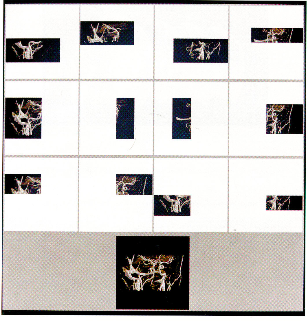
We used three different data sets for our tests. The uorticity data set is a 256x256256 voxel CFD data set, computed on a CM-ZOO, showing the onset of turbulence. The hectd data set is the now classic UNC Chapel Hill CT head at a size of 128x128128. The vesseldata set is a 256x256~128 voxel hlagnetic Resonance Angiography (MRA) data set showing the vascular structure wjthin the brain of a patient. Plate 1 illustrates the compositing process described in Figure 4: using the images generated with this vessel data set. Similarly, each column shows the images from one processor. while the rows are the phases of the compositing algorithm. The final image is displayed at the bottom.
5.1 CM-5
We performed multiple experiments on the CM-5 using partition sizes of 32, 64, 128, 256 and 512. When these tests were run, a 1024 partition was not available. All times are given in seconds. For the vorticity data set, we show COIIIplete timing results in Table 1 and the speedup graph in Figure 5. The times shown are the broadcast time (data) and the maximum times for all the nodes for the two steps of the core algorithm: the rendering step (rend) and the cornpositing step (camp), followed by the actual communication component (comm) in the compositing step and lastly the image gathering time (send). Note that the speedup was measured for the core algorithm and it is a function of the 32 node running time. Due to limited space, for the Ilead and vessel data sets, we show only the corresponding speedup graphs in Figure 6 and 7, respectively.
Looking at Table 1, it is easy to see that rendering time

dominates the process. It should be noted that this implementation does not take advantage of the CM-5 vector units. We expect much faster computation rates in the ren-

derer when the vectorized code is completed. As there is no communication in the rendering step, one might expect

linear speedup when utilizing more processors. As can be seen from the three speedup graphs, this is not always the case due to the load balance problems. The uotticity data

set is relatively dense (i.e. it contains few empty voxels) and 2.4.2
IJnlike a massively parallel supercomputer dedicating uniform and intensive computing power, a network computing environment provides nondedicated and scattered computing cycles. Thus, using a set of high performance workstations connected by an Ethernet, our goal is to set up a volume rendering facility for handling large data sets and batch animation jobs. That is, we hope that by using many workstations concurrently, the rendering time will decrease linearly and we will be able to render d&a sets that are too






size opt
data re11d

camp

642

1282 COlnm send rend CO,,,P conllll send 1 rend




Table 32 89.87 0230:3?3 0.0137 0.0013 0.0161 :3.1446 0.047:3 0.00:30 O.OGO8 I I 12.334 1: CM-5 Results 64 93.518 0.3995 0.0125 0.0008 0.0168 1.5974 0.0406 0.002G 0.0615 13.:31:3:3 I 128 83.185 0.2072 0.0101 O.OOOG 0.0187 0.8247 0.0300 0.0018 o.oti57 :3.X305 I 256 94.3x 0.1116 0.0101 0.0005 0.0218 0.4086 0.0279 0.0012 0.0687 I %I58 512 49.157 0.0597 0.0094 0.000:3 0.0280 0.2041 O.lLx35 0.001 I 0.07:34 I 0.806:3 on the Vorticitv Data Set backups. The four IBM’s were all OII the same suhnet, while the remaining nodes lie on different suhnets. Thus, we expect the co&munication performance for the one, two and four machines to be better t.han for the eight or more.
In a heterogeneous environment, it is less meaningful to use spccdup graphs to study the performance of our algorithm and implementation. Thus in Figure 8, 9 and Ill, for the rendering step and t,he compositir& step. varying the number of workstations and the image size, we display the maximum times from the tests on the vorlicity, hcc~d and vessel data sets, respect.ively. Note that we use a Iog scale along the y axis. The solid lines show the time for both steps and the dotted lines show the time for the rendering step only.
In a shared computing environment, the communication costs are highly variable due to the use of the local Ethernet There are many shared with hundreds of other machines. factors that we have no control over that are influential to and our algorithm. For example, an overloaded network other users’ processes competing wit.h our rendering process for CPU and memory usage could greatly degrade. the per-

formance of our algorithm. Improved performance could bc achieved by carefully distributing the load to each computer

according to data content, and the computer’s performance COLII- ,x+ well as its average usage by other users. !vioreover, munications costs are expected t.o drop with higher speed

interconnection networks (e.g. FDDI) and on clusters isolated from the larger local area network.

Unlike the CM-~‘S results, tests on workstations show that. the communication component is the dominant factor in the compbsiting costs. This can be seen by comparing the solicl

lines with the dotted lines in the graphs. On the average. communication takes about 97% of t.he overall cornpositing

time. However, while using eight or fewer workstations, the rendering time still dominates the compositing time in most cases. Again, the significant performance degradation for

rendering smaller images is due to the overhead cost,s associated -with the rcndcring and compositing steps. These

graphs exclude the data distribution and image gather times. These times varied greatly, due to the variable load on the shared Ethernet. The data distribution times varied from 17

seconds to 150 seconds while the image gather times varied from an average of .06 seconds for a 64x64 image to a high

of 8 seconds for a 512x512 image. Preliminary results with PVM 3.1 indicate much lower comnionicatiotls costs.
therefore exhibits nearly linear speedup. On the other hand, both the head and the vessel data sets contain many empty VOX& which unbalance the load and therefore do not exhibit the best speedup. Figure 5 demonstrates that for the uorticity data set, our implementation achieves very good speedup for all image sizes except 64x64. The rendering of the 64x64 image exhibits less speedup than larger image sizes due to overhead costs associated with the rendering and compositing steps. In particular, the compositing step showed a speedup of only 1.46 when going from 32 nodes to 512 nodes. For all image resolutions above 64 x64, the overall speeclup was nearly the same.
The broadcast time includes the time it takes to read the data over NFS at Ethernet speeds on a loaded Ethernet. The broadcast time for the 512-node case is substantially less than for the smaller partitions because while the timings were being gathered for partitions smaller than 512 nodes, the other partitions were also running other jobs causing both disk and Ethernet contention. The image gathering time (send) is the time it takes for the nodes to send thei; composited image tiles to the host. As can be seen, the image gathering time is only slightly slower for larger partitions which have more image-tiles. Both of these &es will

be mitigated by use of the. parallel storage and the use of the HIF’F’I frame buffer.

5.2 Networked 6 Conclusions \Ve have presented a parallel volume ray-tracing algorithm for a massively parallel computer or a set of interconnected

workstations. The algorithm clividcs both the comput.ation and memory load across all processors and can therefore be

used to render data sets that are too large to fit into the memory system of a single uniprocessor. i parallel (binnryswnp) compositing method was developed to combine the

independently rendered results from each processor. The binary-swap compositing method has merits which make it

particularly suitable for .mas.sively parallel processing. First, while the parallel compositing proceeds, the decreasing image size for sending and compositing makes the overall com-

pbsiting process very efficient. Next, this method alwavs keeps all processors busy doing useful work. Finally, it ‘is

simple to implement with the use of the k-D tree structure described earlier.
The algorithm has been implemented on both the (:M-5

and a network of scientific workstations. The (:M-5 impleWorkstations
For our workstation tests, we used a set of 32 high performance workstations. The first four machines wcrc IBM RS/GOOO-550 workstations equipped with 512 MB of IIICIW ory. These workstations are rated at 81.8 SPECfp92. The next 12 machines were HP9000/730 workstations, some with 32 MB and others with 64 MB. These machines are rated at 86.7 SPECfp92. The remaining 16 machines were Sun Spare-10/30 workstations equipped with 32 MB, which are rated at 4.5 SPECfp92. The tests on one, two and four workstations used only the IBM’s, The tests with eight and 16 used a combination of the HP’s and IBM’s. The 16 Sun’s were used for the tests on 32. It was not possible to assure absolute quiescence on each machine because they are in a shared environment with a heavily used Ethernet and large files systems. During the period of testing there was a network traffic from NSF activity and across-the-net tape

20





render+composite render only 14 -
.

12

10

Speedup 10 Time 8
(set>

6
1 4

2


0 3264

5: CM-5 Figure I 0.1 0
128 Number Speedup for the I’orticity Data 4 0 512 256 of Processors
Figure Set.
I8: F’VM I
8 12 Number Results I I
16 20 24 of Processors 28 I I on t,he Vorticity 32 Dilta Set.

I6

12 128x128 -E-

10 512X.512 -e-

Speedup render+composite
render only 100 14 -
. . .
10 Time 8
(=I

6
1

4

2 0.1 0


| 0 | 0.1 | |
|---|---|---|
| 0 3264 | 128 2.56 512 | |
| Number of Processors | ||
| Figure 15: CM-5 | Speedup for the Head Data Set. | Figure |



512x.512 0 512 Figure Set.
of Processors 28 Results on the Head Data Set.





8 24 16 20
of Processors 28 9: PVhl I I
12 Number I
32 10 Time (set)
0 3264

Figure 7: CM-5 128 Number Speedup 256 of Processors for the 0 5 I 2 Velssel Data Set. Fignre

4 10: PVM 12 Number Results on the Vessel Data Sel.
32




PI GEIST, G., AND S~NDERAM, V. Network-ba5ed mentation showed good speedup characteristics out to the

largest available partition size of 512 nodes. Only a small fraction of the total rendering time was spent in communi-

cations, indicating the success of the parallel compositing method. Several directions appear ripe for further work. The host data distribution, image gather, and display times

are bottlenecks on the current C:M-5 implementation. These bottlenecks can be alleviated by exploiting the parallel I/O

capabilities of the C:M-5. Rendering and compositing times on the C:M-5 can also be reduced significantly by taking advantage of the vector units available at each processing node.

We are hopeful that real time rendering rates will be achievable for medium to high resolution with these improvements.

Performance of the distributed workstation implementation could be further improved by better load balancing. In a heterogeneous environment with shared workstations, Iin-

ear speedup is difficult. A simple approach is to do static load balancing. The data subdivision can be done unevenly,

taking into account the predicted capacity on each machine to try to balance the load. Alternatively, the data can be subdivided into a larger number of equal sized subvolumes

and the more capable machines can be assigned more than one subvolume. The later approach has the advantage that

it can be generalized to a dynamic load balancing approach: divide the data into many subvolumes and assign them to processors in a demand driven fashion. The finer subdi-

vision of the data volumes would improve load baIancing during rendering at the cost of some additional compositing

time due to more levels in the cornpositing tree.
PI HANRAHAN, P. Three-Pass Affine Transforms for Vol-
ulue Rendering. Computer Graphics 24, 5 (1990). Spccial issue on San Diego workshop on Volume Rendering. PI LEVOY,
IEEE PI LEVOY, Display hl.
of Surfaces from Volume Graphics Efficient A CM Transactions 261.
arLd Data. (May .4pylications Ray Tracing on G’raphics of Volume 9, 3 (July Data. 1990): 245- PO1 MA, K.-L., C:OHEN, IM., AND PAINTER, J. VoIuuie
Seeds: A Volume Explorat.ion Technique. The Journal of Visualization 135-140. Pll MA, K.-L.,
sualization and Computer Animation 2 (1991), AND PALIVTER, J. S. Parallel Volunle ViWorkstations. Computers and Graphics on 17, 1 (1993). P31 MACXERRAS, P. A Fast Parallel Marching (.:ubes 11u-
plcmentation on the Fujitsu APlOOO. Tech. Rep. TR(.S-92-10, Department of (-:omputer Science, Australian National University, 1992.
[I31 MONTANI, C:., PEREGO, R., AND SCYOPIGNO, R. Paral-
lel Volume Visualization on a Hypercube Architecture. .In 1992 Workshop on Volume Visualization (1992).

pp. 9-16. Boston, October 19-20.
[I41 NIEH, J., AND LEVOY, M. Volulne Rendering on Scal-

able Shared-Memory MIMD Architectures. Ill 199,” Workshop on Volume Visualization (1992), pp. 17-24.

Boston, October 19-20.
The M RA vessel data set was provided by the MI RL at the University of Utah. The vorticity data set was provided by Shi-Yi C:hen of T-Div at Los Alamos National Laboratory. David Rich, of the AC:L, and Burl Hail, of Thinking Machines, helped tremendously with the C:M-5 timings. The Alpha-l and CSS groups at the IJniversity of Utah pro-

vided the workstations for our performance tests. Thanks go to Elena DriskiIl for comments on a draft of this paper.

This work has been supported in part by NSF/AC:ERC: and NASA/IC:ASE.
for C:omputer-Generated Pic- [I51 PHONG, B. Illumination
tures. f?ornrnun. .4C11f 18, 6 (June 1975), 31 l-317. [161 PORTER, T., AND DUFF, T. C:ompositing
In Proceedings pp. 253-259.
ages. of SIG’G’RAPH Digital Iul‘84 (July 1984),

[171 SCZHFGDER, F’., AND SALEM, J. B. Fast Rotation of
Volume Data on Data Parallel Architectures. In Proceedings of Visualization’9f (October 1991), pp. 50-57.
References

Multidimensional IJsed for Associative Searching.

(September 1975), 509-517.
Binary Search Trees Cotnrnur. ACM 18, 8 1181 SCXSGDER, P., AND STOLL, G. Data Parallel Volume
Rendering as Line Drawing. In 199,” Workshop on volurne Visualization (1992), pp. 25-31. Boston, October 19-20. PI C:ATMULL, E., AND SMITH, A. R. 3-D Transformations

of Images in Scanline Order. (1980), 279-285.
hl. C’omp?:t~~. 1988), 39-37.
Acknowledgments PI BENTLEY, J.
Concurrent C:omputing on the PVM System. Concurrency: 4, 4 (June 1992), 293-312. Practice and Expt&nce Computer Graphics 14, 3 I191 THINKING MAC:HINES C:ORPORATION. T/ie
C’omsction Machine

PI DOC:TOR, L., AND TORESORG, J. Display Techniques
for Octree-Encoded Objects. IEEE Cornput. Graphics

and Appl. 1 (July 1981), 29-38.
CM-5 Technical Summary, 1991.
PO1 THINKING MAC:HLUES C:ORPORATION. CYMMU Rejer-
ence Manual; Preliminary 3.0 Beta, February [41 FXHS, H., ABRAM, G., AND GRANT, E. D. Near Real-

Time Shade Display of Rigid Objects. In Proceedings oj SIGGRAPH ‘83 (1983), pp. 65-72.
Docunentation for Versiorz 1993. WI VZINA, C;., FLETCHER, P. A., AND ROBIZRTSON,
Volume Rendering on the MasPar .MP-1. In 1992 Workshop on volume Visualization (1992), pp. 3-

P. K.
[51 FUCHS, H., POULTON, J., EYLES, J., GREER, T.,
GOLDFEATHER, J., ELLSWORTH, D., MOLNAR, S.,

TI.RK, C., TEBBS, B., AND ISRAEL, L. Pixel-Planes 5: A Heterogeneous Multiprocessor Graphics System Us-

ing Processor-Enhanced Memories. Computer Graphics “9, 3 (July 1989), 111-120.
PI


22 Yoo, T., NEIIMANN, IJ., FUC:HS, H., PIZER, S., C:~:LLLF, T., RHOADES, J., AND WHITAKER, R. Direct Visualization of Volunle Data. IEEE Computer Graphics and Applications (July 1992), 63-71.















....... ._ ._
..... ....
_ _
.......
.. .:.‘...- .. :. ... ” .- __ _ . . _ .










c

Plate 1: Illustration of the parallel image cornpositing process using the vessel dat.a

set. Each column sllows the images from one processor, while the rows arc the phases of the cornpositing algorithm. The iirlal image is displayed at the bott.om.


Ma, Painter,
Hansen, Krogh


_ _
